Gamma-Alpha
The following examples all simulates the \gamma\rightarrow\alpha transformation of a ternary steel model alloy including iron (Fe), carbon (C) and manganese (Mg).
| Example | Description |
|---|---|
| [T02_20_FeCMn_E_GammaAlphaIsotherm_2D_Lin]](#files) [T011_T02_21_FeCMn_E_GammaAlphaIsotherm_2D_TQ]](#files) | Demonstration of the difference between MICRESS® simulations with and without coupling to Thermo-Calc™. Both examples are concentration-coupled (either linearized phase diagrams or database use) and demonstrate the use of the "seed-undercooling" nucleation model. |
| [T02_22_FeCMn_E_GammaAlphaIsothermPara_2D_TQ]](#files) [T02_23_FeCMn_E_GammaAlphaIsothermParaTQ_2D_Lin]](#files) | Important for solid-state transformations in systems with slow and fast diffusing elements is the use of the NPLE (non-partitioning, local equilibrium) redistribution model. Both examples use the para-equilibrium models instead. |
| [T02_27_FeCMn_E_GammaAlphaStress_2D_Lin]](#files) | shows how stress coupling can be included. |
The following examples are variations of the [T011_T02_21_FeCMn_E_GammaAlphaIsotherm_2D_TQ]](#files) model.
| Example | Description |
|---|---|
| T02_24_FeCMn_E_GammaAlphaCementite_2D_TQ | utilizes full coupling to a thermodynamic database. |
| T02_25_FeCMn_E_GammaAlphaCementite_2D_TQ+Lin | demonstrates the application of a combination between linearized phase diagrams and coupling to a thermodynamic database. Furthermore, cementite is added as third solid phase. |
| T02_26_FeCMn_E_GammaAlphaPearliteEff_2D_TQ | demonstrates the use of the "diffuse" effective phase model for pearlite. |
Alloy
| Alloy system | Fe-C-Mn (FeCMn.Ges5) |
| Composition | Group A
|
| Transition | solid phase transition |
Group A
Group A demonstrates how to use MICRESS® for simulation of solid state transformations like the alpha to gamma transition. Characteristic for simulation of solid state transformations is the necessity to define an initial microstructure which is typically not needed in case of solidification. In this case, 9 initial grains of ferrite are positioned with user-defined center coordinates and radii. Voronoi construction is used to obtain a typical grain structure without overlapping or holes. The specific input data can either be chosen manually for small numbers of grains or taken from specific tools like "Random_Grid". Alternatives for definition of initial grain structures are random generation or reading from experimental microstructures or prior MICRESS® simulations.
Transformation is calculated at a constant temperature of 1023 K (750 °C) where the alpha (fcc) phase is thermodynamically stable. But during the phase transformation, the dissolved elements C and Mn are redistributed, reducing the driving force for transformation. While C is a fast diffusor and can move away from the interface, Mn diffuses too slow in the time-scale of the transformation and thus must be overrun (nple) or trapped (para/paratq). This fact that the diffusion profiles of Mncannot be spatially resolved makes it necessary to use specific models for solute redistribution which avoid artefacts of the standard redistribution model. In these examples, the conditions are chosen such that the different redistribution modes nple and para/paratq are leading to substantially different transformation rates, because in case of nple the pile-up of the element Mn in front of the moving interface is taken into account for calculation of the driving-force, while in case of para or para-tq it isn't.
The purpose of the 4 different versions of T010_Gamma_Alpha is to demonstrate on one hand the differences when using linearised phase diagram data and fix Arrhenius-type diffusion coefficients versus thermodynamic and diffusion databases, and on the other hand the redistribution models nple versus para or paratq. For the first type of comparison ([T02_20_FeCMn_E_GammaAlphaIsotherm_2D_Lin]](#files) vs. [T02_21_FeCMn_E_GammaAlphaIsotherm_2D_TQ]](#files) and T02_22_FeCMn_E_GammaAlphaIsothermPara_2D_TQ vs. T02_23_FeCMn_E_GammaAlphaIsothermParaTQ_2D_Lin) it is demonstrated how input is specified. When comparing the simulation results it turns out that there are substantial differences. The reason here is that the different redistribution modes nple and para/paraTQ lead to strongly different local tie-lines which cannot be reasonably approximated by a single linearized description. The second type of comparison (T02_20_FeCMn_E_GammaAlphaIsotherm_2D_Lin vs. T02_22_FeCMn_E_GammaAlphaIsothermPara_2D_TQ and T02_21_FeCMn_E_GammaAlphaIsotherm_2D_TQ vs. T02_23_FeCMn_E_GammaAlphaIsothermParaTQ_2D_Lin) shows strong differences in the transformation kinetics due to the different redistribution behaviour of Mn.
It should be noted that the numerical and physical parameters used in these examples are not necessarily correct or validated by literature! The user who intends to build up own simulations based on these examples takes the full responsibility for choosing reasonable values!
Group B
Group b) consists of a single example and demonstrates how to include elastic stress in the simulation of the gamma-alpha transformation. note that in this case stress is calculated only for the output time steps. The contributions to the driving force are neglected here.
Group C
Group c) includes cementite as a further solid phase into the simulation. The spatial resolution is adapted for the gamma-alpha reaction and thus too low for resolving individual pearlite lamellae. Two different strategies are compared how pearlite is represented: In T02_24_FeCMn_E_GammaAlphaCementite_2D_TQ, a high number of individual cementite particles are nucleated, resembling a phase mixture with consistent phase fractions and compositions but incorrect microstructure. On the other hand, T02_26_FeCMn_E_GammaAlphaPearliteEff_2D_TQ uses a diffuse phase model which represents pearlite as a continuous phase mixture.
T02_25_FeCMn_E_GammaAlphaCementite_2D_TQ+Lin is added for demonstrating how to proceed if a certain phase (cementite in this case) is not contained in the thermodynamic database. Here, only the interaction between gamma and alpha is simulated using the database while the interactions of these two phases with cementite are defined by linearized phase diagrams (in this case using the "linTQ" format).
Results
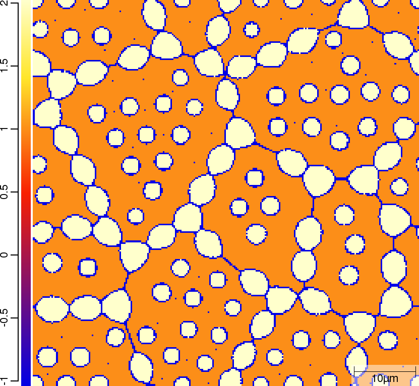
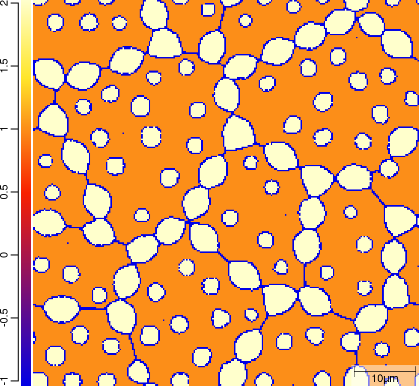
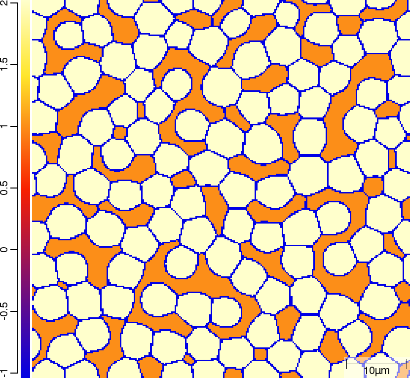
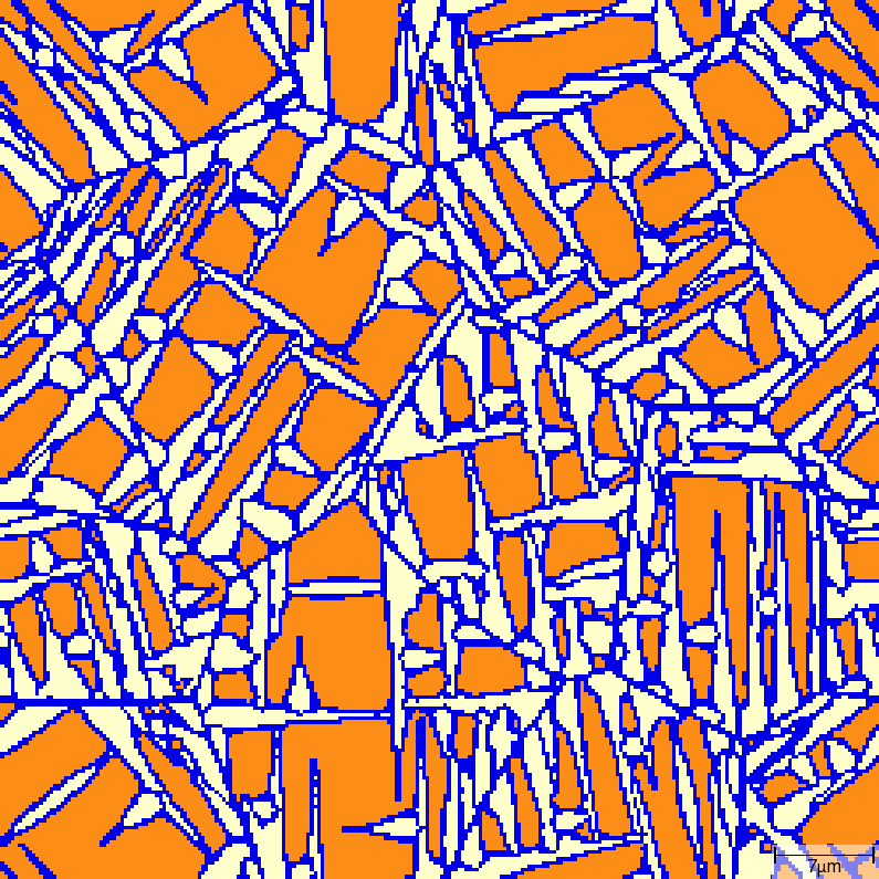
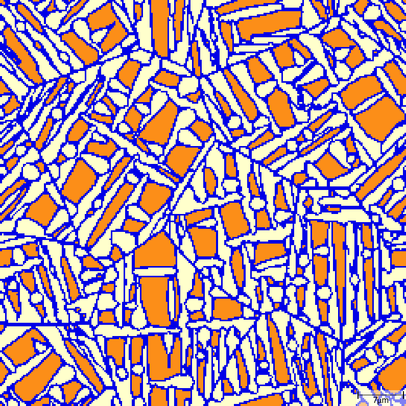
Group A
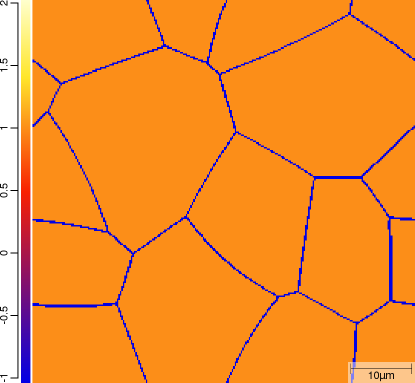
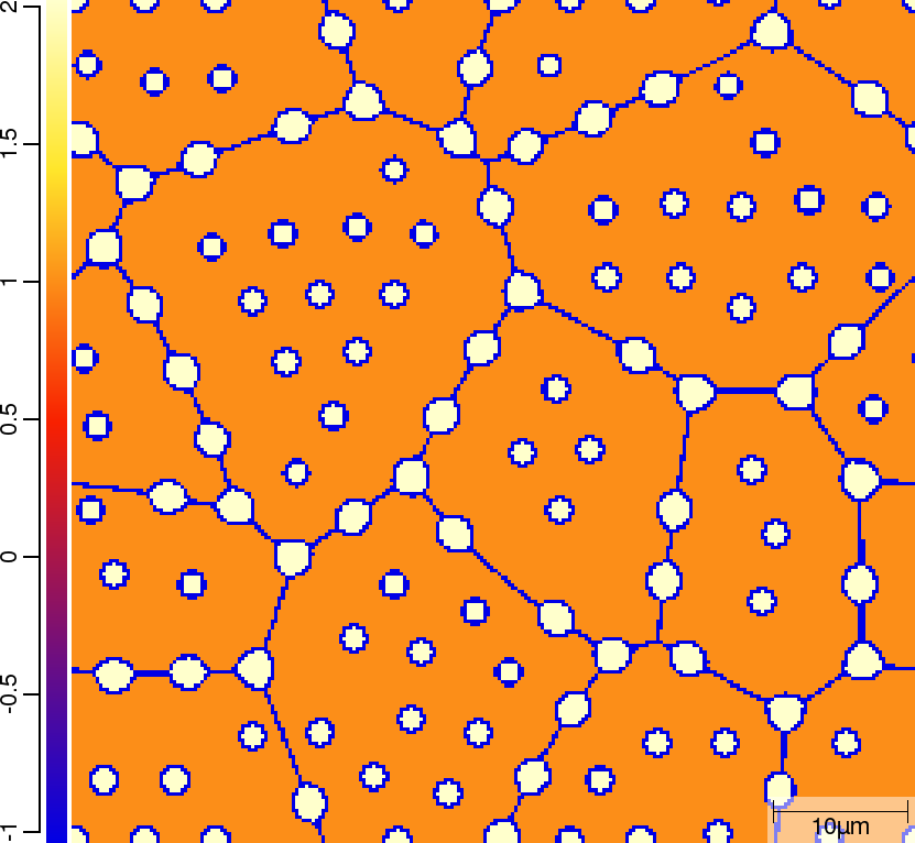
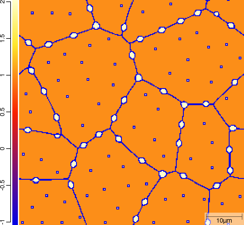
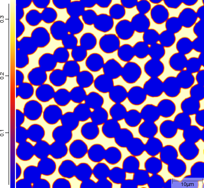
Phase transition sequence
| T02_20_FeCMn_E_GammaAlphaIsotherm_2D_Lin | T02_21_FeCMn_E_GammaAlphaIsotherm_2D_TQ | T02_23_FeCMn_E_GammaAlphaIsothermParaTQ_2D_Lin |
|---|---|---|
| t=0\rm{s} | ||
 |  |  |
| t=50\rm{s} | ||
 |  | 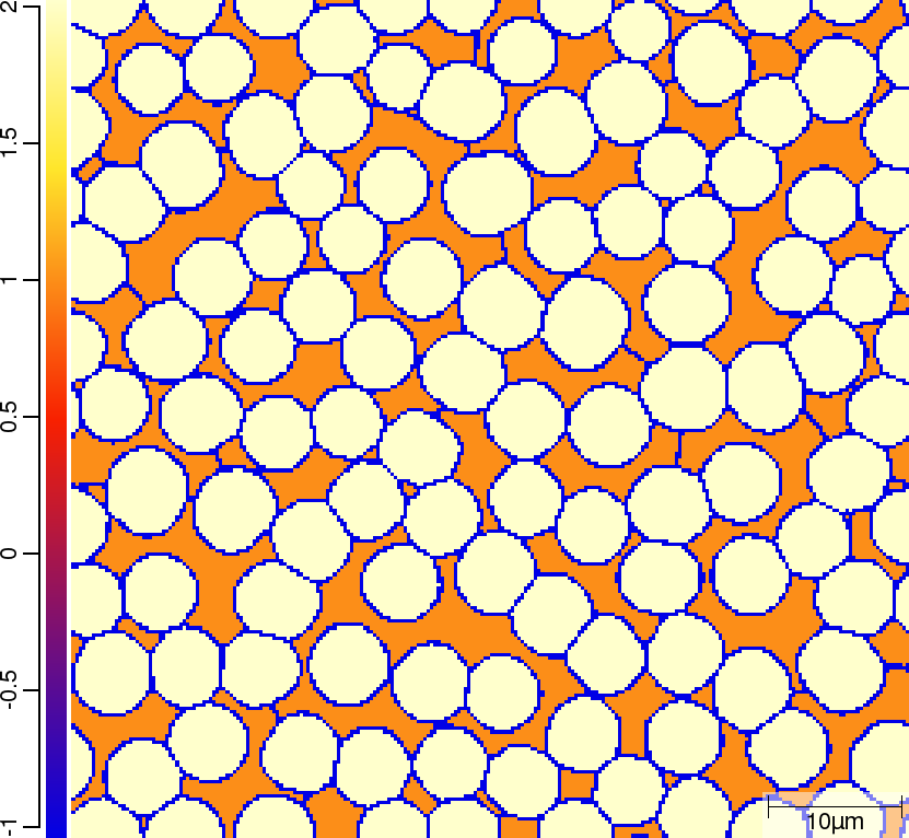 |
| t=300\rm{s} | ||
 |  |  |
Carbon (C) composition at t=50\rm{s}
| T02_20_FeCMn_E_GammaAlphaIsotherm_2D_Lin | T02_21_FeCMn_E_GammaAlphaIsotherm_2D_TQ | T02_23_FeCMn_E_GammaAlphaIsothermParaTQ_2D_Lin |
|---|---|---|
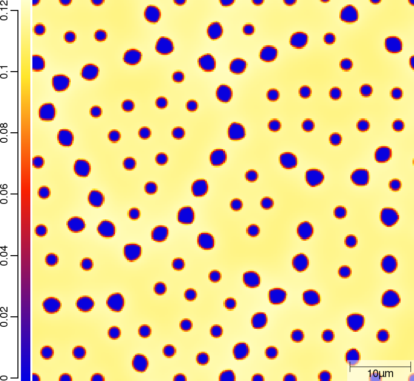 | 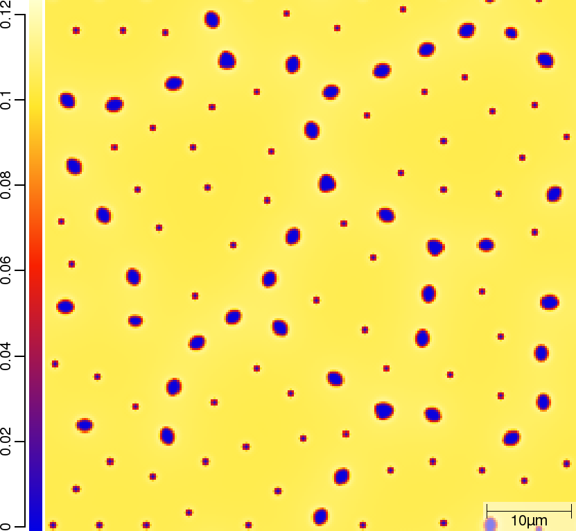 |  |
Group B
Phase transition sequence
-1: interface, 0: unassigned, 1: gamma; 2: alpha; 3: cementite
| T02_25_FeCMn_E_GammaAlphaCementite_2D_TQ+Lin | T02_24_FeCMn_E_GammaAlphaCementite_2D_TQ |
|---|---|
| t=0\rm{s} | |
 |  |
| t=6.5\rm{s} | |
 |  |
| t=13\rm{s} | |
 |  |
| t=35\rm{s} | |
 |  |
Carbon (C) and Manganese (Mg) composition at t=35\rm{s}
| T02_25_FeCMn_E_GammaAlphaCementite_2D_TQ+Lin | T02_24_FeCMn_E_GammaAlphaCementite_2D_TQ | ||
|---|---|---|---|
| C | Mg | C | Mg |
 |  |  |  |
Group C
T02_27_FeCMn_E_GammaAlphaStress_2D_Lin phase transition sequence
-1: interface, 0: unassigned, 1: gamma; 2: alpha; 3: cementite
| t=0\rm{s} | t=6\rm{s} | t=10\rm{s} | t=15\rm{s} |
|---|---|---|---|
 |  |  |  |
T02_27_FeCMn_E_GammaAlphaStress_2D_Lin von Mises stress
| t=0\rm{s} | t=6\rm{s} | t=10\rm{s} | t=15\rm{s} |
|---|---|---|---|
 |  |  |  |
Acicular growth
T02_30_FeC_E_GammaAlphaAcicularA_2D_Lin phase transition sequence
| t=7\rm{s} | t=8\rm{s} |
|---|---|
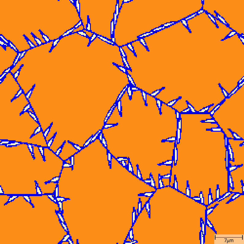 | 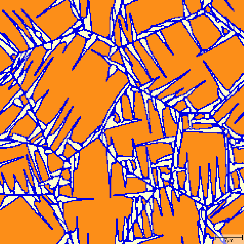 |
| t=9\rm{s} | t=10\rm{s} |
|---|---|
 |  |
Links
- T02_20_FeCMn_E_GammaAlphaIsotherm_2D_Lin
- T02_21_FeCMn_E_GammaAlphaIsotherm_2D_TQ
- T02_22_FeCMn_E_GammaAlphaIsothermPara_2D_TQ
- T02_23_FeCMn_E_GammaAlphaIsothermParaTQ_2D_Lin
- T02_27_FeCMn_E_GammaAlphaStress_2D_Lin
- T02_30_FeC_E_GammaAlphaAcicularA_2D_Lin
- T02_24_FeCMn_E_GammaAlphaCementite_2D_TQ
- T02_25_FeCMn_E_GammaAlphaCementite_2D_TQ+Lin
- T02_26_FeCMn_E_GammaAlphaPearliteEff_2D_TQ