Phase Interaction
When defining the phase interactions between two phases, the user may define either standard interactions or use some special models. E.g. in case of grain growth, the user may decide to use the particle pinning model, the solute drag model or recrystallization for the description of the grain boundary migration. Figure 1 shows the difference in the development of the average grain radius with time for the first two models mentioned above and normal grain growth.
The particle pinning model and the solute drag model will be described in more detail in the next sections.
Apart from these mesoscopic models, there are also advanced options for defining a dedicated redistribution behaviour of solute in the interface. Selecting this option allows the activation of the NPLE-model, the paraequilibrium model or an antitrapping current (ATC) for each element (see phase diagram input).
Figure 1
Normal grain growth vs. the particle pinning and the solute drag models

Particle pinning model ("Zener model")
The term particle pinning describes the effect of small particles on the movement of grain boundaries. If the driving force for the movement of the grain boundary (typically the curvature) is not high enough to overcome the attractive interactions with the particles, the grain boundary is pinned and will not move any more. Thus, the grain size may be reduced to a much lower value by the effect of particle pinning. In practice, particle pinning is an important mechanism in preventing softening of materials at high temperature due to grain growth. The particle pinning model implemented in MICRESS® is a meso-scale model which takes into account the microscopic particle pinning effect without treating the individual particles explicitly. According to the Zener model, a critical pinning force P^* \sim 3 \sigma c / r is defined, where \sigma is the particle surface energy, c is the particle concentration and r the particle radius (Figure 2).
Figure 2
Figure 3.10 The particle pinning model
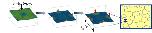
If the driving force p exceeds the critical driving force, the grain boundary will still move, but with a lower velocity. This velocity has been simulated for discrete particles using MICRESS® (Figure 2). The velocity curves can be described by an effective mobility which is implemented in the mesoscopic MICRESS® particle pinning model. The user has to provide the critical pinning force p^* in units of a critical pressure (MPa) (default option) or a critical curvature (1/{\mu m}) and a minimal mobility.
For grain growth, the driving force for grain boundary movement consists of the grain boundary curvature and the force balance at the triple junctions. In general, this driving force decreases with the average grain size. But especially the force balance at the triple junctions is not directly linked to the grain size. Therefore, with the particle pinning model, abnormal grain growth may be observed, e.g. one huge grain continues growing while the smaller ones are already pinned.
From a theoretical point of view, the minimal mobility parameter should be zero. But in many cases, even if pinning occurs, still a very slow movement of the grain boundaries is observed, e.g. due to particle ripening. MICRESS® gives the user the possibility to account for that by specifying a minimal mobility >0.
Table 1 shows that using the particle pinning model instead of normal grain growth leads to different results. In the figure above, a clear tendency towards abnormal grain growth can be seen in the simulation where the particle pinning model has been used.
Table 1
Grain growth simulation with and without particle pinning
| Time | Particle pinning disabled | Particle pinning enabled |
|---|---|---|
| 0s | 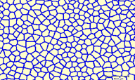 |  |
| 1000s | 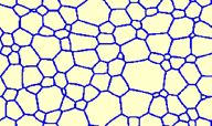 | 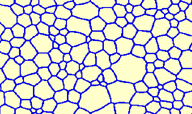 |
| 2000s | 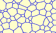 | 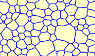 |
| 3000s | 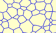 | 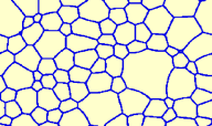 |
Solute drag model
The solute drag effect can be described as follows: in case of attractive interaction between the grain boundary and dissolved impurity atoms, the solute atoms will be concentrated at the boundary. When the boundary moves, the solute atoms will try to remain on the boundary, i.e. the boundary has to drag its impurity load and can only migrate as fast as its slowly moving impurities. If the actual velocity v is lower than the critical velocity \nu^*, the solute atoms will stay with the interface, which is then referred to as a loaded interface and is characterised by a decreased mobility. If the actual velocity \nu is larger than the critical velocity \nu^*, the solute atoms cannot follow the movement and there is a free interface formed, characterised by a high mobility. Thus, the impurity drag model uses a two step velocity dependent mobility of the grain boundary for description of the interaction of the grain boundaries with solute atoms (Figure 3).
Figure 3
The solute drag model
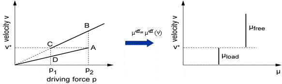
Important parameters here are the critical velocity \nu^* and the drag factor, by which the mobility of the grain boundary is reduced due to the drag effect. In order to prevent numerical fluctuations around the critical velocity, a transition range \Delta V has to be specified: In the range between \nu^* - 0.5 \cdot \Delta V and \nu^* + 0.5 \cdot \Delta V, there is a linear transition between the reduced mobility \mu^* drag factor and the normal mobility \mu.
Anisotropy of interfacial energies and mobilities
If at least of two interacting phases has been defined as anisotropic or faceted, the interfacial properties can be defined as anisotropic, i.e. as function of the interface normal vector \vec{n} = (n_x,n_y,n_z) transformed into the coordinate system of the anisotropic grain. Two alternative model versions can be chosen to describe weak (non-faceted) anisotropy: The default standard model and the new harmonic_expansion model.
The standard anisotropy model is based on predefined anisotropy functions, listed in Table 2. The specific choice of the anisotropy function depends on the crystal symmetry which the user has defined for the anisotropic phase, as previously described in topic Phase -- Anisotropy.
Table 2
Standard anisotropy functions predefined in MICRESS®
| Cubic | Anisotropy function | 2-D equivalent |
|---|---|---|
| Stiffness | 1 - \delta_{\sigma^*} 4(n_x^4 + n_y^4 + n_z^4 - 0.75) | 1 - \delta_{\sigma^*} \cos 4\phi |
| Mobility | 1 + \delta_{\mu} 4(n_x^4 + n_y^4 + n_z^4 - 0.75) | 1 + \delta_{\mu} \cos 4\phi |
| Hexagonal | Anisotropy function | 2-D equivalent |
|---|---|---|
| Stiffness | (1 - \delta_{\sigma^*} (-n_x^6 + 15n_x^4 n_z^2 - 15n_x^2 n_z^4 + n_z^6) - \vert\delta_{\sigma^*}\vert (n_y^6 + 5n_y^4 - 5n_y^2)) \cdot (1 - n_y^2 + n_y^2 f_y) | 1 - \delta_{\sigma^*} \cos 6\phi |
| Mobility | (1 - \delta_{\mu} (-n_x^6 + 15n_x^4 n_z^2 - 15n_x^2 n_z^4 + n_z^6) - \vert\delta_{\mu} \vert (n_y^6 + 5n_y^4 - 5n_y^2)) \cdot (1 - n_y^2 + n_y^2 f_y) | 1 - \delta_{\mu} \cos 6\phi |
| Tetragonal | Anisotropy function | 2-D equivalent |
|---|---|---|
| Stiffness | a_{\sigma^*}^{cubic} \cdot (1 -n_z^2 + n_z^2 f_z) | z elongated cubic |
| Mobility | a_{\mu} ^{cubic} \cdot (1 -n_z^2 + n_z^2 f_z) | z elongated cubic |
| Orthorhombic | Anisotropy function | 2-D equivalent |
|---|---|---|
| Stiffness | a_{\sigma^*}^{cubic} \cdot (1 -n_z^2 + n_z^2 f_z -n_y^2 + n_y^2 f_y) | z elongated cubic |
| Mobility | a_{\mu} ^{cubic} \cdot (1 -n_z^2 + n_z^2 f_z -n_y^2 + n_y^2 f_y) | z elongated cubic |
The user can specify anisotropy coefficients \delta_{\sigma^*} and \delta_{\mu} in the range of \delta \in [0,1]. A typical value for \delta_{\mu} in cubic metal systems equals 0.05. Elongation factors can exceed the value of 1, but have to be positive. Table 3 illustrates the standard anisotropy functions for different choices of symmetry and coefficients.
Table 3
Examples of standard anisotropy functions with specific choice of coefficients
| Cubic | Hexagonal | Tetragonal | Orthorhombic | |||
|---|---|---|---|---|---|---|
 |  |  |  |  |  |  |
| \delta=0.25 | \delta=0.25 f_y=1 | \delta=0.25 f_y=0 | \delta=0.25 f_z=1.2 | \delta=0.25 f_z=0 | \delta=0 f_z=0 | \delta=0.25 f_y=0.6 f_z=0.8 |
 |  |  |  |  |  |  |
| \delta=-0.25 | \delta=-0.25 f_y=1 | \delta=-0.25 f_y=0 | \delta=-0.25 f_z=1.2 | \delta=-0.25 f_z=0 | \delta=0 f_z=2 | \delta=-0.25 f_y=0.6 f_z=0.8 |
It is important to note that the static anisotropy is defined in the standard model with respect to the interfacial stiffness \sigma^* instead of with respect to the interfacial energy \sigma. The use of the the interfacial stiffness in the phase-field equation allows a direct matching to to the modified Gibbs-Thomson equation for anisotropic interfaces which reads: \nu = \mu (\Delta G - \sigma\kappa) with \nu being the velocity in normal direction, \mu the mobility, \Delta G the driving force and \kappa the curvature, for more details see 1. In the 2-D case, the interfacial stiffness can easily be related to the interfacial energy by \sigma^* = \sigma + d^2 \sigma / d\phi^2. However, this is not possible in 3-D, where curvatures in two different spatial directions have to be distinguished. Here, the stiffness model simply represents a pragmatic solution to consider a static anisotropy based on the same function as for the kinetic anisotropy. For a correct treatment of quantitative interfacial energy data in 3-D, the alternative anisotropy model which can be selected by the optional keyword harmonic_expansion is recommended.
The harmonic-expansion model is especially helpful for 3-D simulations and also to incorporate quantitative interfacial data from experiments or Molecular Dynamics simulation. Here, the anisotropy functions are formulated by linear combination spherical harmonics selected in accordance with the crystal symmetry. The implemented harmonic functions are listed in Table 4:
Table 4
Combinations of spherical harmonic function defined in MICRESS®
| Symmetry | Anisotropy function |
|---|---|
| Cubic | a=1+\epsilon_{c_1}Y_{c_1}+\epsilon_{c_2}Y_{c_2} |
| Hexagonal | a=1+\epsilon_{66}Y_{66}+\epsilon_{20}Y_{20}+\epsilon_{40}Y_{40}+\epsilon_{60}Y_{60} |
| Tetragonal | a=1+\epsilon_{20}Y_{20}+\epsilon_{40}Y_{40} |
| Orthorhombic | a=1+\epsilon_{20}Y_{20}+\epsilon_{40}Y_{40} |
| Symmetry | Spherical harmonics |
|---|---|
| Cubic | Y_{c_1} = 4(n_x^4+n_y^4+n_z^4) - 3 Y_{c_2} = n_x^6+n_y^6+n_z^6 + 30 n_x^2 n_y^2 n_z^2 |
| Hexagonal | Y_{66} = \frac{\sqrt{6006}}{64\sqrt{\pi}} (-n_x^6 + 15n_{yx}^4 n_z^2 - 16 n_x^2 n_z^4 + n_z^6) Y_{20} = \frac{\sqrt{5}}{4\sqrt{\pi}} (3n_y^2 - 1) Y_{40} = \frac{3}{16\sqrt{\pi}} (35n_y^4 -30n_y^2 + 3) Y_{60} = \frac{\sqrt{13}}{32\sqrt{\pi}}(231n_y^6 - 315 n_y^4 + 105 n_y^2 -5) |
| Tetragonal, Orthorhombic | Y_{20} = \frac{\sqrt{5}}{4\sqrt{\pi}} (3n_z^2 - 1) Y_{40} = \frac{3}{16\sqrt{\pi}} (35n_z^4 -30n_z^2 + 3) |
The contributions of individual harmonic functions are illustrated in Figure 1. The user can combine these contributions by the specific choice of the individual coefficients \epsilon, which allows modeling of complex, manifold anisotropy functions. The choice of harmonic function for tetragonal and orthorhombic symmetry is only preliminary and shall still be extended according to future users demands.
Table 5
Contribution of individual harmonic functions with positive and negative coefficient
| 1+\epsilon_{c_1} Y_{c_1} | 1+\epsilon_{c_2} Y_{c_2} | 1+\epsilon_{20} Y_{20} | 1+\epsilon_{40} Y_{40} | 1+\epsilon_{60} Y_{60} | 1+\epsilon_{66} Y_{66} |
|---|---|---|---|---|---|
 |  |  |  |  |  |
| 1-\epsilon_{c_1} Y_{c_1} | 1-\epsilon_{c_2} Y_{c_2} | 1-\epsilon_{20} Y_{20} | 1-\epsilon_{40} Y_{40} | 1-\epsilon_{60} Y_{60} | 1-\epsilon_{66} Y_{66} |
|---|---|---|---|---|---|
 |  |  |  |  |  |
In contrast to the standard model, the static anisotropy is in the harmonic_expansion model formulated with respect to the interfacial energy, which enters the free energy functional. The detailed derivation of the anisotropic phase-field equations is described in section 3.3 in 1.
Faceted anisotropy
If at least one of the two interacting phases has been defined as faceted, the phase interaction will be modeled as faceted. In this case, the interfacial stiffness \sigma^*(\theta) and the interfacial mobility \mu(\theta) are evaluated as functions of an angle \theta, denoting the angle between the interfacial normal vector and the nearest normal facet vector \vec{f}_n.
An arbitrary number of facet vectors and corresponding coefficients can be defined. Note that in theory, faceted aniostropy are characterized by forbidden (instable) regions with negative stiffness, causing a discontinuous orientation change between neigbouring facets. Diffuse interface models, however, require regularized anisotropy functions with strictly positive stiffness to allow for a sharp, but numerically continuous transition. In Micress, different faceted anisotropy models have been tested; the current and recommended is named faceted_c (or simply faceted), but all former versions faceted_a, faceted_b and antifaceted are still available.
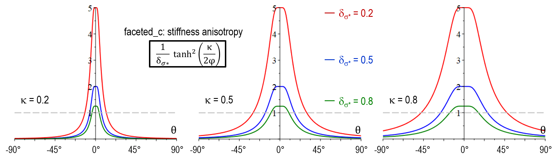
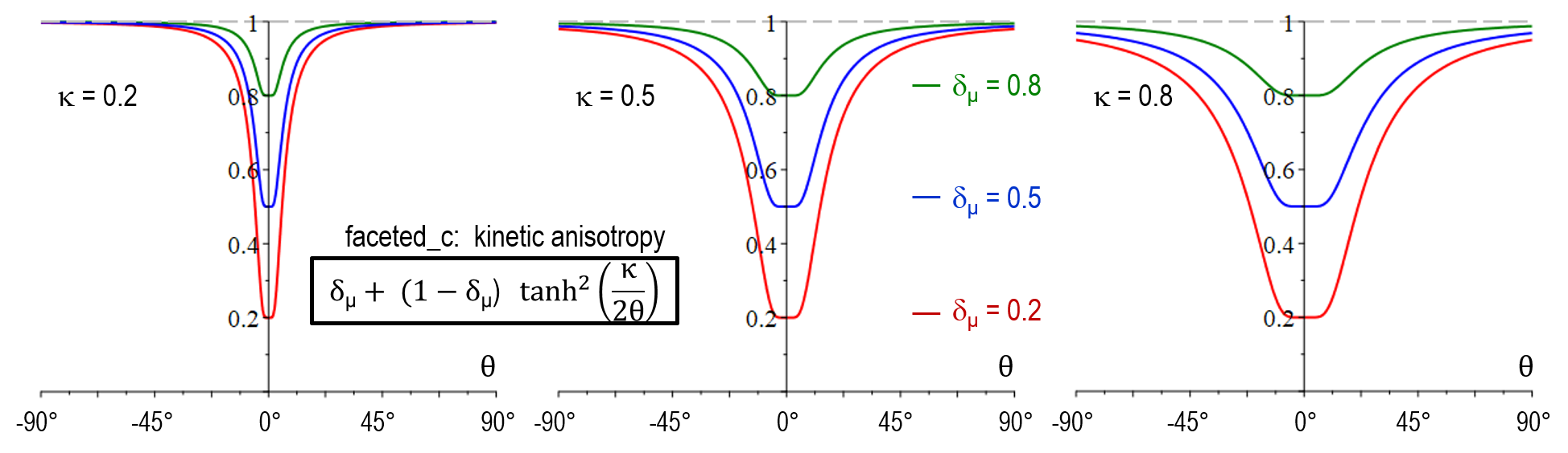
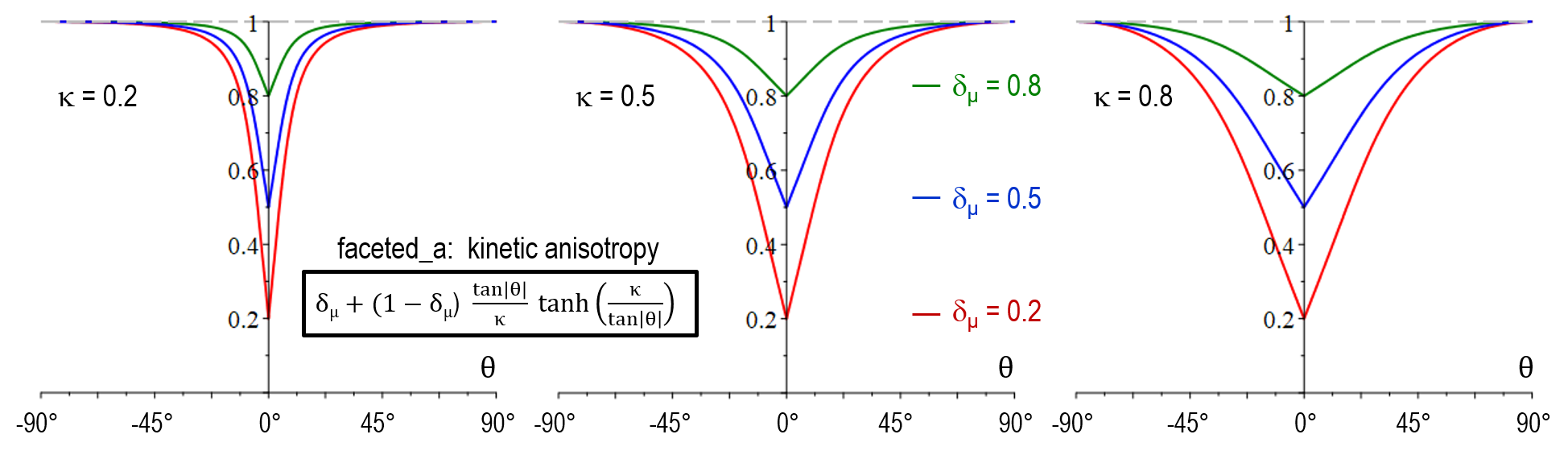
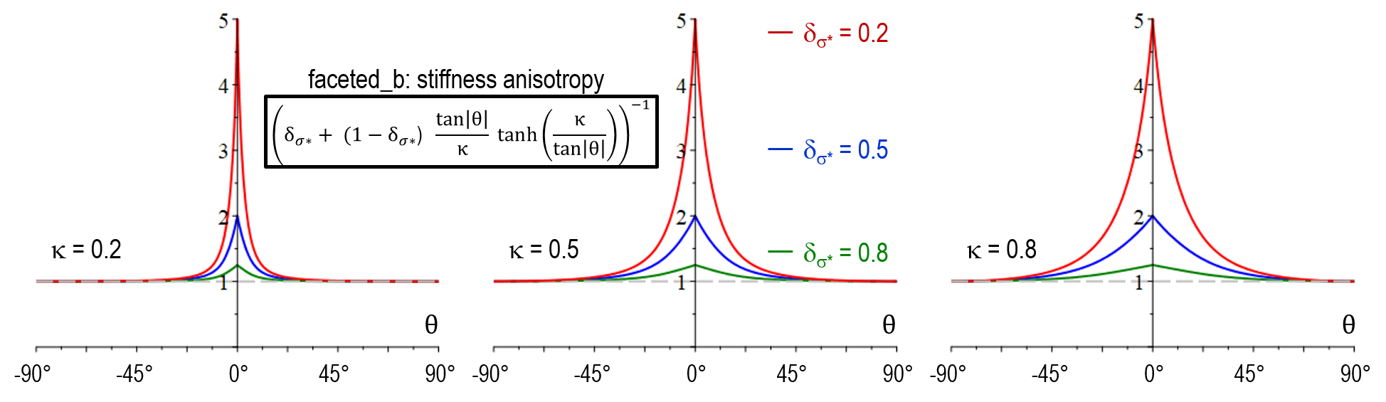
The strength of anisotropy is determined by the anisotropy coefficient \delta_{\sigma^*} for the stiffness, and \delta_\mu for the mobility, both defined in the range from >0 to 1. It is important to note that \delta_{\sigma^*/\mu} = 1 corresponds to isotropic behavior and the anisotropy increases with decreasing cofficient. In direction of the normal facet-vector (\theta = 0), the stiffness function has its maximum a_{\sigma^*}(0) = 1/\delta_{\sigma^*} and the mobility function its minimum a_\mu(0) = \delta_\mu. For \vert \theta \vert> 0, the stiffness changes to a minimum and the mobility to a maximum. The width of this transition can be adjusted by the parameter \kappa.
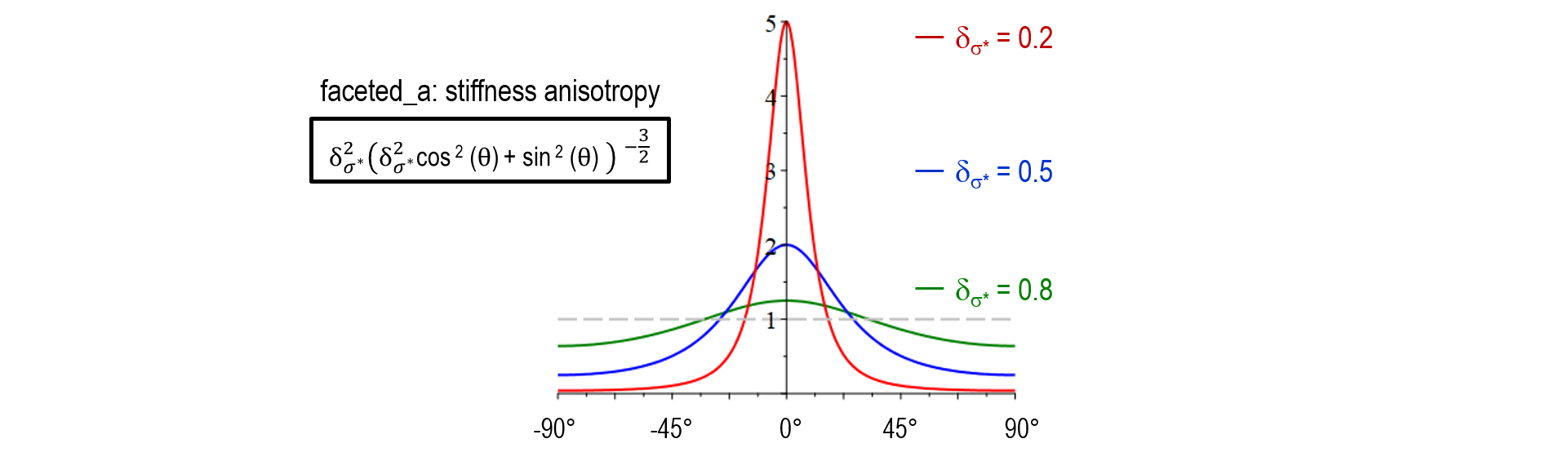
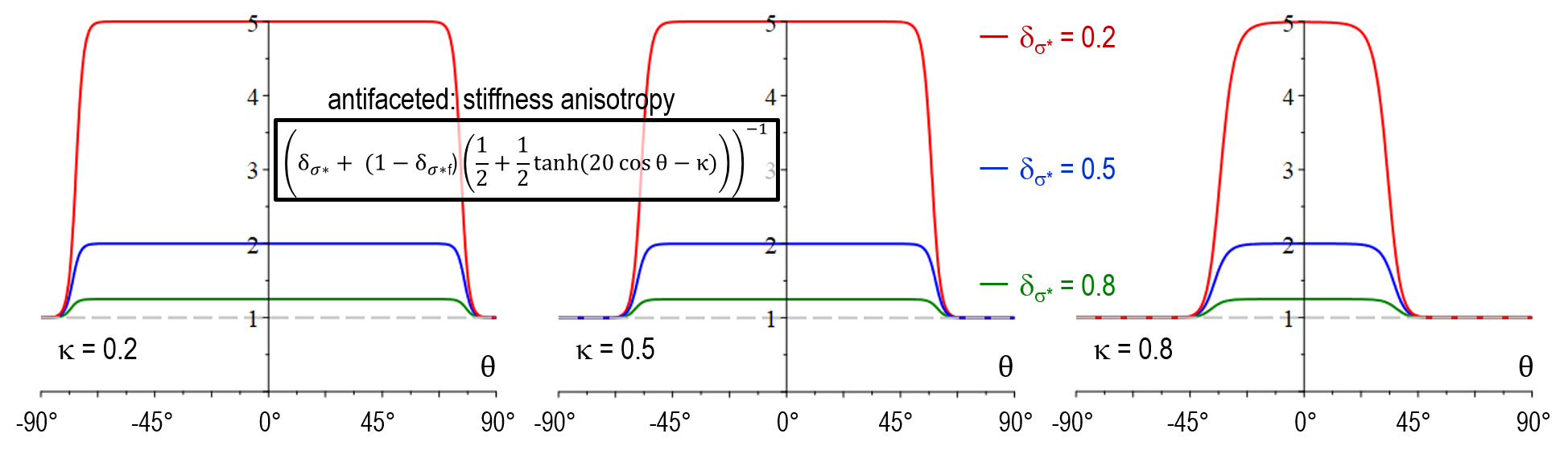
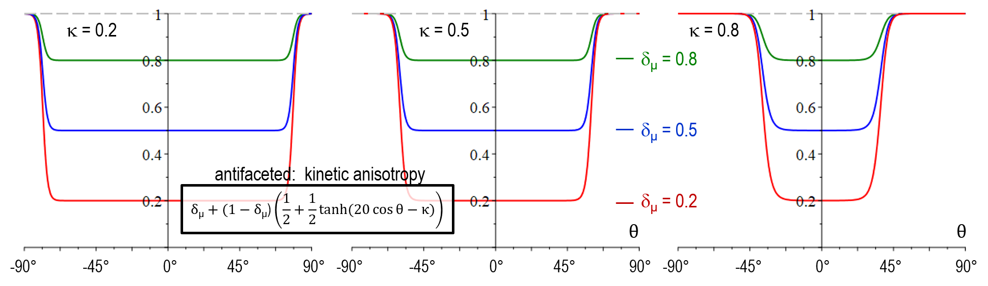
As illustrated below, the stiffness function in model version faceted_a did not yet allow for adjustment of the transition width (no \kappa-dependency). Another major shortcoming was that a_{\sigma^*}(\theta) increased with \delta_{\sigma^*} for large values of \theta which resulted in in a wrong selection at the edges behavior between neighboring facets of different strength. An additional novel feature of faceted_c is that the physical singularity at \theta = 0 was smoothed out, accounting for the numerical uncertainty in the evaluation of \theta. A problem of both faceted_a and faceted_b was that small numerical errors in the vicinity of \theta = 0 resulted in large artefacts and hindered to model a sharp transition in arbitrary directions. The antifaceted model represented a former pragmatic solution to simulate thin plates which should -after introduction of faceted_c- not be necessary anymore.
| New model faceted(_c) | Anisotropy function |
|---|---|
| Stiffness anisotropy a_{\sigma^*}(\theta) | \frac{1}{\delta_{\sigma^*}} \tanh^2(\frac{\kappa}{2\theta}) |
| Mobility anisotropy a_{\mu}(\theta) | \delta_\mu + (1-\delta_\mu) \tanh^2( \frac{\kappa}{2\theta}) |
| Former model faceted_a | Anisotropy function |
|---|---|
| Stiffness anisotropy a_{\sigma^*}(\theta) | \delta^2_{\sigma^*} (\delta^2_{\sigma^*} \cos^2\theta + \sin^2\theta)^{-3/2} |
| Mobility anisotropy a_{\mu}(\theta) | \delta_\mu + (1-\delta_\mu) \frac{\tan \vert \theta \vert}{\kappa} \tanh(\frac{\kappa}{\tan \vert \theta \vert}) |
| Former model faceted_b | Anisotropy function |
|---|---|
| Stiffness anisotropy a_{\sigma^*}(\theta) | [ \delta_{\sigma^*} + (1-\delta_{\sigma^*}) \frac{\tan \vert \theta \vert}{\kappa} \tanh(\frac{\kappa}{\tan \vert \theta \vert})]^{-1} |
| Mobility anisotropy a_{\mu}(\theta) | \delta_\mu + (1-\delta_\mu) \frac{\tan \vert \theta \vert}{\kappa} \tanh(\frac{\kappa}{\tan \vert \theta \vert}) |

| Former model antifaceted | Anisotropy function |
|---|---|
| Stiffness anisotropy a_{\sigma^*}(\theta) | [ \delta_{\sigma^*} + (1-\delta_{\sigma^*}) (\frac{1}{2} + \frac{1}{2} \tanh(20\cos \theta -\kappa))]^{-1} |
| Mobility anisotropy a_{\mu}(\theta) | \delta_\mu + (1-\delta_\mu) (\frac{1}{2} + \frac{1}{2} \tanh(20\cos \theta -\kappa)) |
Phase diagrams
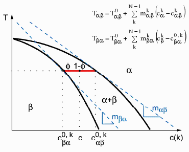
Using linearised phase diagrams
The input required for applying linearised phase diagrams includes the reference temperature at which the linearisation was performed, the entropy of transformation, the concentration of each component in the considered phases, and the corresponding slopes.
Use linearised phase diagram description if:
- no thermodynamic database is available
- the system is simple and quite linear (e.g. FeC)
- the considered process is (almost) isothermal
- you need to reduce the risk of numerical instabilities
- simulation time and memory usage are critical
- thermodynamic noise is problematic
- MICRESS® is used for teaching purposes or qualitative modelling
Figure 4
A linearised phase diagram
Coupling to thermodynamic databases
Components with concentration 0
It is not possible to include a component with concentration 0 in a simulation with TQ-coupling, e.g. when more components than needed are defined in the GES5 file. A composition of 0 is only allowed for stoichiometric phases, and then the corresponding composition needs to be specified for another phase which has solubility for this phase. This is not astonishing because a composition of 0 would correspond to an infinitely low entropy and thus an infinitely high driving force for dissolution of such a component from another phase.
A better procedure in such cases is either to use a GES5 file without this element or is to specify a non-zero but sufficiently small value for this composition. But the user should be extremely careful, because this small value can nevertheless be important for numerical reasons and can affect performance!
When to choose coupling to thermodynamic databases?
Choose coupling to thermodynamic databases if:
- a full thermodynamic description including all phases and elements is available
- systems are complex (technical alloys, ternary or higher, more than two phases)
- a wide temperature range is addressed
- realistic behaviour is required
- you do not like to rack your brain about thermodynamics!
Global vs. local thermodynamic description
While for local thermodynamic description (keyword database or database local in the definition of the phase diagram input per phase pair) each interface cell has its own thermodynamic description which is obtained from the database when the interface cell is newly formed or when the description is updated, with global thermodynamic description (keyword database global) only one such description is used for a complete interface between two grains. The local thermodynamic description is default and should be used as such because it is safer and more exact. At triple junctions, consistent descriptions for all pair-wise interactions are assured, because the same mixture composition in the considered grid cell and identical phase fractions are used while updating the data from database (it is also taken care that all interfaces in a triple or higher junction are updated even if only updating for one phase pair is requested.
If a global thermodynamic description is used for a certain phase pair, this consistency cannot be assured. But, as compensation, a mostly significant reduction of the calculation effort for this phase pair is achieved (which can be checked in the .TabTQ output). This often gives the possibility to afford using a smaller updating interval which may compensate for the loss of numerical stability. The use of global thermodynamic descriptions can be worthwhile for phase interactions between precipitations which are small and thus do not feel much differences in composition or temperature with their surroundings. This option may also be successfully used if numerical noise inside an interface which is connected to the phase diagram description is a problem, e.g. at the very end of a solidification simulation or during Ostwald ripening of particles of thermodynamically difficult phases like MC carbides.
Which updating schemes should be chosen?
There are presently 5 different updating schemes for thermodynamic data available:
- Global updating interval
- Updating interval per phase pair
- Critical effective temperature deviation per phase pair (
automatic) - No explicit updating (
none)
The most simple and reliable method is using a global updating scheme. By this way, a complete updating of all thermodynamic descriptions is assured and the computational effort can be controlled. The smaller the updating interval, the more accurate are the results but the higher is the computational effort. The user should use a value which is small enough not to affect considerably the results but high enough to fulfil his performance requirements.
Using updating per phase pair should be considered if certain phase pairs need special care, and the strong performance loss connected with a small global updating interval has to be avoided.
Note: If updating per interface and global updating is combined, extra effort can be created if the intervals are no exact multiples. Also, in case of pure updating per phase pair and local thermodynamic descriptions, an extra effort is to be expected for triple and higher junctions if no exact multiples are used for the update frequencies (consistency of triple junctions!).
A smart method is to update thermodynamic descriptions only when needed. i.e. when the local conditions change sufficiently. An effective temperature deviation can be calculated for each interface cell using the temperature and concentration change since the last updating of this grid cell. With the updating method relying on a critical temperature deviation, the complete interface is updated if for one interface cell this limit is exceeded (updating only this single cell would produce huge noise which could even destroy the interface!). The main disadvantages of this method are that it can be quite difficult to figure out a reasonable value for the critical temperature deviation and that the computational effort is very difficult to predict
No explicit updating does not necessarily mean that the simulation is incorrect: All newly formed interface cells are automatically up to date, and if an interface is moving fast enough, the thermodynamic description is implicitly updated. Depending on the type of simulation (e.g. steady state growth using the moving frame option), no explicit updating may be needed