Numerical Parameters
2-D simulations of 3-D structures
Very often memory usage turns into a problem for the performance of 3-D simulations which are expensive concerning both time consumption and memory usage. In such cases it is often reasonable to perform 2-D simulations of the given 3-D structures. But how to choose the correct 2-D parameters in order to obtain a structure that resembles the original 3-D one the best way? How close are the simulation results of one and the same structure, once simulated as 2-D and once as 3-D? The following cases allow you to perform a 2-D simulation:
-
No curvature in 1-D, e.g. planar solidification front and lamellar eutectic structure: 2-D simulation is correct
-
One axis is predominant, e.g. due to a temperature gradient: 2-D simulation deviates from the 3-D one within a small factor in the order of \sqrt{2} (Figure 1)
-
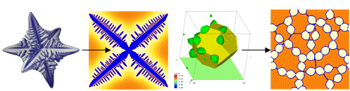
No axis is predominant (see Figure 5).
Figure 1
One axis is predominant
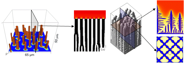
Figure 2
No axis is predominant
Grid resolution and interface mobilities
The number of grid cells, i.e. the resolution for a given domain size, strongly affects the simulation time. Assuming that diffusion is the performance bottleneck, one can expect a factor of 16 in simulation time, if the value of \Delta X is divided by 2! Therefore it is very important to find the optimal resolution.
In general, the resolution is high enough, if a small change in \Delta X does not change the results. In order to make a systematic study it is important to reduce the problem (temporarily) to the smallest representative size (taking advantage of all possible symmetries). With this small domain size it should be possible to get down to the really high resolutions where the results do no longer depend on the resolution. For this test simulation, all critical physical parameters (diffusion coefficients, interfacial energies, interface mobility) must be already adjusted because they would change the test results. To quantify the differences, one can choose, e.g. the phase fraction of the growing phase or the temperature, if latent heat is used.
The procedure would be the following: starting from the highly resolved test simulation, one would increase stepwise \Delta X and compare the chosen quantity vs. time (e.g. phase fraction), observing from which \Delta X the \Delta t_x gets substantially different. Then, one would go one step back and use the corresponding \Delta X for the big simulation.
Unfortunately, in many cases one would still be in a \Delta X range where performance is poor. In that case, one could go one step further: typically, a too low resolution for a diffusion-limited phase transformation leads to an artificial solute trapping and increased front kinetics. To a certain degree, one can try to compensate for that by reducing the interface mobility. As long as the development of the phase fraction can be corrected in this way, and the morphology is also retained (a different morphology earlier or later will also affect the fraction-time curve!), there is no reason not to do that!
If one is willing to invest even more calibration effort, one can use additional numerical parameters like the DG options (averaging length etc.) to even better adjust to the correct interface kinetics and phase morphologies.
Related to that is also the choice of a reasonable value of the interface thickness. If performance is critical, one can go down to 3.5 cells without deteriorating the curvature evolution too much.
Of course, all these measures may decrease the exactness of the microstructure predictions for a given domain size. But, if due to the better performance a larger domain can be simulated, the exactness of the overall result may be increased!
The proper choice and meaningful adjustment of the numerical parameters are crucial for the successful numerical prediction of the results. The most critical parameters for numerical stability are:
- grid resolution: must be high enough to resolve the diffusion profiles, related to the diffusion coefficients and the growth velocity of the surface and the curvatures of the finest microstructure, expected from it;
- interface mobility: must be high enough to allow diffusion-controlled growth without kinetically slowing down the interface.
This means that using very high resolution and high interface mobilities would automatically result in stable simulations. Indeed this is true in most cases, but it is not practical because it results in extremely high calculation times! For example, increasing grid resolution by a factor of 2 in a 2-D simulation will result in a factor of 4 (8 for 3-D) for the simulation time, if the simulation is limited by interface related load (high proportion of interface in the calculation domain), or by a factor of 16 (32 for 3-D), if diffusion is time-limited! Increasing the interface mobility proportionally reduces the phase-field time step and thus increases the simulation time.
As a general approach for finding proper numerical parameters:
-
Try to use the smallest size of the simulation area which still represents your problem. After finding suitable parameters you can apply them to larger domains or more complex problems.
-
Reduce the problem to only one interface between two phases. Optimising different phase interaction at a time will produce confusion!
-
Use the automatic time stepping option to get rid of the time-step as an additional numerical parameter.
-
Do not use physical parameters for optimising numerical stability! If you do not know all of them, make guesses and stick to them, until later you can calibrate them by comparison of stable simulations to experimental data.
Depending on whether one needs quantitative or just qualitative results, and whether one can afford the high resolution, the following three empirical approaches can be used.
Approach 1: Qualitative work
Choose a resolution for which you have the feeling that you can afford (in terms of calculation time). Start with a guessed mobility value. If the simulation crashes or shows instabilities, lower the mobility value until you get a stable run. Look at the driv output to see whether the movement of the interface is slowed down strongly by the choice of your mobility! If that is the case, the grid resolution is not fine enough. Try again with a smaller value. On the other hand, if the simulation runs properly with your first guess of the mobility and resolution value, try to reduce the mobility or increase the grid spacing to make your simulation even faster.
Approach 2: Full resolution of the microstructure and diffusion profiles
If you want to be sure that the choice of the grid resolution and interface mobility does not affect the results of your simulation, you need to check quantitatively the growth velocity of the interface. This can be easily done by plotting one of the phase fractions vs. time (TabF) or the temperature vs. time (TabL), if release of latent heat used. Then you can check quantitatively the growth kinetics for different parameter settings. The way to proceed is the following.
Start from a given grid resolution and modify systematically the interface mobility. You will experience that growth kinetics will get faster with increasing the interface mobility, as long as you are in the range of too low mobilities. If you further increase the interface mobility depending on the grid spacing, you will get the following behaviour:
- grid spacing is too large: The growth rate of the interface will increase further until you end up in numerical instabilities.
- grid spacing is small enough: The growth rate will reach a plateau and remain constant even for higher Interface mobility values.
Once you observe such a plateau, you can be sure that (at least from numerical reasons and assuming diffusion-limited growth!) your results are quantitative. Unfortunately, there are only few cases where you can afford to solve your problem completely with that high resolution. In most cases you have to proceed to Approach 3.
Approach 3: Quantitative without fully resolving microstructure and diffusion profiles
A way to get the right kinetics even if you cannot afford the high resolution you would need for complete resolving the microstructure and diffusion profiles is to use the interface mobility to calibrate the growth kinetics. This necessarily means that you need to know the exact kinetics of your process either from experiments or by getting it from a high resolution simulation via Approach 2, using the smallest possible calculation domain which still represents your simulation problem.
Calibration is just done by variation of the interface mobility for the given (too large) value of the grid spacing and comparing (via TabL or TabF output) with the reference simulation (or experiment). This is not always possible if the morphology of the low-resolution simulation is very different to the real one. In that case, you should try to use the averaging of the driving force across the interface to match better the morphology. You can adjust the averaging length of the driving force separately for each phase interaction. In this way, in many cases you will be able to perform low-resolution simulations without getting all microstructure details but with the appropriate growth kinetics.
As shown, it is quite a bit of work to perform quantitative simulations with MICRESS®, if there is no access to infinite computational power or if the problem is not extremely simple. But keep in mind that in many cases you may be just interested in knowing how a system reacts on changes of a physical parameter, or due to the lack of physical parameters you anyway need to calibrate your simulation to experimental results. Then, it is often not necessary to perform a perfect adjustment of the transformation kinetics to get a valuable insight into the problem by simulation.
iface and nTupel
In most cases, the iFace and nTupel parameter values are adjusted automatically. Under special conditions one might wish to be able to control the field sizes in a better way. This may be in the following cases:
-
the user is interested in having a static list size. Then, the second optional parameter should be 0.
-
the calculation begins with a lot of grains (e.g. grain ripening). Starting with 0 as initial size would lead to a high number of increasing list actions during initialisation. This could take some extra time!
-
the user is interested in keeping the list size as small as possible. In that case, the allocated size can be adjusted to the actual size. This can be achieved by a proper specification of the second and third parameter.
Example 2 means for iFace that if less than 80% of the allocated iFace-Field is used, it will be reduced so that 90% of it is used after the reallocation. On the other hand, if in the case of a growing iFace list 100% usage is reached, then the iFace field is increased so that afterwards 90% are used. The default values are 0.50 and 0.75 respectively (iFace and nTupel).
Example 1
List size optimisations
...
# Phase field data structure
# ------------------------------------
# Coefficient for dimension of field iFace
1.0  0
# Coefficient for dimension of field nTupel
0.5  0
...
Example 2
List size as small as possible
...
# Phase field data structure
# --------------------------
# Coefficient for dimension of field iFace
1.0 0.8 0.9
# Coefficient for dimension of field nTupel
0.5 0.7 0.85
...
Phase minimum phMin
The phase minimum (phMin, at the very end of the input file) is a purely numerical parameter which defines the fraction (phase-field parameter) below which an interface cell is assumed to convert to a bulk cell. If the fraction of a phase is below this value, the concentration of the small rest amount is frozen into the other phase(s) which is (are) present in this cell. Consequently, high values of the phase minimum increases artificial solute trapping.
Small values of phMin reduce this effect, but may require smaller phase-field time steps for not producing instabilities related to segregation, and thus slow down the simulation. This is included automatically into the automatic time step function.
However, if a new phase appears in a grid cell, it has at least the fraction corresponding to the value of the phase minimum. In cases where the new phase has a stoichiometric composition much higher than the actual composition in the matrix phase, there may be not enough solute of this component contained in the grid cell, e.g. if the value of phMin is too high.
In most cases, a value of 10^{-4} can be recommended. Lower values down to 10^{-12} can be used if stoichiometric components with extreme concentration differences are involved (like precipitation of carbides from an extremely low carbon matrix).