Nucleation
In practice, inoculants are often added to technical alloy melts which serve as nucleation agents during solidification. They help to achieve a smaller grain size and to suppress columnar growth. Even if no active inoculation is done, impurities, dislocations or the roughness of the interface structures can lead to nucleation phenomena in all types of technical processes.
Unfortunately, apart from the "seed density model" for heterogeneous nucleation from an inoculated melt, no physical models are available for the complex nucleation conditions in technical alloys. Homogeneous nucleation, on the other hand, will typically occur only at very high undercooling and under extremely clean conditions, like in experiments with levitated drops.
Thus, besides the physically based "seed density model" for heterogeneous nucleation, MICRESS® provides the user with a pragmatic nucleation model based on a critical undercooling or critical RX energy or critical mean dislocation density (depending on the adopted model variant) which can be further specified with respect to the type of seed positioning, the temperature range, the matrix and substrate phases, the nucleation rate etc. and which allows the user to mimic the complex nucleation circumstances found in technical alloys or processes.
Seed undercooling model
Using the seed undercooling model, a new seed is set if the local undercooling at a nucleus position exceeds a predefined critical nucleation undercooling. The local undercooling depends on the local composition and temperature.
In general, the MICRESS® nucleation models are designed for micro-scale simulations and not for the nano-scale, i.e. there is no model for the prediction of homogeneous nucleation based on thermal fluctuations for the critical seed formation.
Seed density model
This model describes nucleation from the melt, triggered by small seeding particles which may be added intentionally or which may exist as impurities. Essentially, the critical undercooling for nucleation \Delta T_n of a given phase on this seeding particle depends on the radius r of the seeding particle and the surface energy \sigma_{sl} of the new phase in the liquid, i.e.
Equation 1
with \Delta S representing the entropy of fusion. Consequently, if a radius-density distribution of the seeding particles is known, depending on the cooling conditions, the model can predict how many nuclei will be formed.
If the different grains of the new phase grow competitively, like in equiaxed solidification, the latent heat released by the growing particles has to be taken into account. The easiest way to do that in MICRESS® is to specify the global volume heat extraction rate as a temperature boundary condition. Thus, the total amount of latent heat is released globally on the whole simulation domain1. A more realistic approach for technical castings is the Iterative Homoenthalpic Approximation2.
The seed density nucleation model implemented in MICRESS® is based on a heterogeneous nucleation model1 similar to the one used by Lindsay Greer. A seed density-radius distribution function has to be specified which is defined stepwise (Figure 1).
Figure 1
Seed density-radius distribution
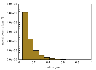
During heat extraction from the melt, the largest particles will nucleate first at an undercooling \Delta T_n defined by their radius r (if complete wetting is assumed or an effective radius is used instead).
The particles start growing and releasing latent heat, while interacting with other potential nucleation precursors. Depending on the heat extraction rate, the amount and sizes of all other seeding particles, the temperature will drop more or less below the liquidus temperature. Thus, the amount of seeds to be activated can be determined. According to the model, the effectiveness of inoculants added for grain refinement is defined by:
- the maximum particle size and
- the particle size distribution.
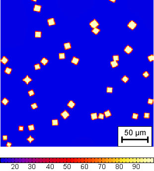
In MICRESS®, the seed density model should be used together with latent heat1 or with coupling to the one-dimensional temperature field (1d_temp)3 in order to allow an interaction of the potential nucleation sites via release of latent heat. Sometimes, it can be used just as a simple way to randomly distribute a given number of nuclei in a defined region. As an example, Figure 2 shows the nucleation of faceted primary Si in an Alusil alloy using the seed density model. In this example, the heat extraction rate dependency of the number and size of primary silicon particles under typical casting conditions is demonstrated.
Figure 2
Nucleation of faceted primary Si in AlSi17Cu4Mg
| \dot{Q}= -62.4\,{\rm J\,cm^{-3}\,s^{-1}} | \dot{Q}= -15.6\,{\rm J\,cm^{-3}\,s^{-1}} |
|---|---|
 |  |
Lognormal distribution
The lognormal distribution function is a kind of probability density function(PDF). It allows to describe the nucleus size distribution that is not symmetrical with regard to the most frequent radius size. In MICRESS®, the lognormal probability density function W(r) in terms of the nucleus radius r\,[{\rm \mu m}] takes the following form:
Equation 2
Here, \hat{\sigma} denotes the standard deviation, which characterizes the width of the distribution. r_{\rm m} is known as the median radius. The cumulative distribution function(CDF) F(r) is obtained by integrating the probability distribution function, i.e.
Equation 3
Here, {\rm erf}(\cdot) indicates the error function. As shown in Figure 3, by the median radius r_{\rm m}, the cumulative distribution function always has a value of 0.5 (or 50\%). The most frequent radius, where the nucleus size frequency has its maximum, r_\rm{mod}\,[{\rm \mu m}] can be calculated by applying its relationship with the median radius and standard deviation as
Equation 4
Figure 3
Lognormal distribution function and the corresponding cumulative distribution function
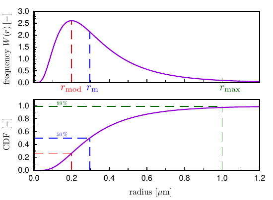
In MICRESS®, it is possible to define the probability density function(PDF) in two equivalent ways. The user should choose one type for his own convenience. By the option lognormal_1 the PDF function is directly determined by the median radius r_{\rm m} and the standard deviation \hat{\sigma} according to Equation 2. By selecting the option lognormal_2, the PDF function is defined by the most frequent radius r_{\rm mod}, and a specific pair of values, namely a nucleus radius r_{\small\rm CDF} and the corresponding CDF value. For instance, the maximal nucleus radius can be found in system cooresponding to a CDF value of 0.99 (or 99\%) could be a convenient choice. In this case, the standard deviation is calculated by using the equation
Equation 5
and the median radius is calculated by inverting Equation 4 as
Equation 6
Shield time and shield distance
The shield time and the shield distance parameters are related. They account for a physical shield effect due to the release of latent heat or solute by a new grain which is not explicitly included in the simulation. This allows the user to set up a pragmatic nucleation scenario if the exact physical background is unknown. Supposed that at a time t a nucleus appears, the parameter shield distance will define a circular area with the diameter r_\text{shield} around the grain. No other grains of the same phase will be allowed to appear on this area within the time interval (t, t+t_\text{shield}). The t_\text{shield} parameter can be defined according to experimental micrographs of the system to be simulated and t_\text{shield} can be evaluated e.g. according to some typical diffusion time scale considerations. The optional parameter nucleation distance defines a radius r_\text{nucleate} that replaces t_\text{shield} only for the time t of nucleation. Choosing r_\text{nucleate} \gt 2 r_\text{shield} helps to distribute nucleation sites more evenly and over multiple time steps.
Diffuse phase model for unresolved eutectic or eutectoid regions
In many cases the length scale of eutectic microstructures is much smaller compared to grains or dendrites, and one may not be able to have both microstructure scales in one simulation. One typical example for that is the pearlite reaction which leads to the formation of lamellae in the submicron range while ferrite and austenite grains are orders of magnitude bigger. Treating pearlite as effective phase with its own phase properties is (at least in multicomponent systems) thermodynamically not consistent. Therefore we follow another approach which treats pearlite as a diffuse phase mixture of cementite and α-ferrite. The optional parameter unresolved, which can be specified in the same line with the phase number for new nuclei, activates this model for the new grain and the corresponding parent grain which must be of the two eutectic phases. These two grains will not form an interface but mix as an extended triple-junction which is diffuse but can have locally different fractions. For further reference check the example T018_GammaAlphaPearliteTQ.dri which is part of the MICRESS distribution.
Advanced grain manipulation using add_to_grain
This option which can also be activated in the same line with the phase number for new grains provides a bunch of possibilities for advanced manipulation of grains. The original intention why this option was included was the possibility to nucleate liquid phase during runtime. In order not to get unphysical grain boundaries inside the liquid phase, new liquid regions have to be formed by grain 0 which per default is already existing (at least in the data structure). Therefore, the task was generally to allow nucleation of grains which already exist, hence the name add_to_grain. Having two or more not interconnected regions with the same associated grain number is nothing exceptional, so there is no reason why this should not be possible. The only side effects are that there will no interface be formed when these regions get in contact later (the same like for categorized grains, see topic Phase - Categorization, and that both regions are associated with the same grain properties like phase number, orientation, shield data, etc. But this latter fact is the reason why the new option provides several interesting possibilities for manipulating existing grains. But first let us have a look on the sub-options which are available with add_to_grains and which must be specified in the following line:
grain_number: The grain number of the new grain is explicitly specified. If this number already exists a second instance of this grain is createdparent_grain: The parent grain (the locally found grain with highest fraction of the substrate phase, or alternatively of the matrix phase if no substrate is defined) is used to define the grain number of the new grain. As this grain already exists at this place, no change is done to the microstructure, but the grain properties of the parent grain are overwritten according to the nucleation parameters.new_set: This seed type opens a new set of instances with the same but before unused grain number
With these three options, a number of smart applications are possible, e.g:
- Nucleation of liquid without formation of unphysical liquid grains
- Nucleation of a set of new precipitates with the same grain number (
new_set). This reduces the total number of grains like thecategorizeoption, but even more efficiently, and thus can greatly improve performance. Please note that due to their common identity, the small grain model may not work correctly (Chapter 3.6.1), andfd_correction(Chapter 2.3) should be used for compensation. - A phase
switch: Using the sub-optionparent_grain, the phase number of an existing grain can be changed to another phase by using the nucleation mechanism. Martensitic transformations which occur instantaneously are a prominent example where this switch may apply. - Removing rest of liquid in solidification is another very useful application of the phase switch: Tiny amounts of remaining liquid often cause serious problems at the end of solidification, typically without being physically meaningful. Switching this remaining liquid (grain 0) to a solid phase is a very simple but effective method to avoid such problems!
- If the simulation of a chain of processes is performed, stored energy or dislocation density due to deformation processes can be applied during run-time or can be added to structures read using the restart functionality.
- Grain orientations can be continuously rotated during simulation by using
parent_grainandparent_relation.
Notes
Not all manipulations which are possible are reasonable!
Phase switches can cause numerical problems if the new phase has solubility restrictions!
-
Ingo Steinbach. Phase-field models in materials science. Modelling and Simulation in Materials Science and Engineering, 17(7):073001, jul 2009. doi:10.1088/0965-0393/17/7/073001. ↩↩↩
-
B. Böttger, M. Apel, J. Eiken, P. Schaffnit, G.J. Schmitz, and I. Steinbach. Phase-field simulation of equiaxed solidification: a homoenthalpic approach to the micro-macro problem - modelling of casting, welding and advanced solidification processes. 2009. MCWASP XII - International Conference on Modeling of Casting, Welding and Advanced. ↩
-
B. Böttger, J. Eiken, and M. Apel. Phase-field simulation of microstructure formation in technical castings - a self-consistent homoenthalpic approach to the micro-macro problem. Journal of Computational Physics, 228(18):6784–6795, oct 2009. doi:10.1016/j.jcp.2009.06.028. ↩