Boundary Conditions
Pressure condition for TQ
When using a database the pressure condition for thermodynamic calculations defaults to the standard of 101325 Pa. To change this parameter switch on TQ volume control (see input section Database) and enter the pressure there. One use is to set the pressure for a system including an oxygen gas phase to the partial pressure of oxygen in air. This pressure is completely independent of any pressures calculated in the flow module.
1-D far field approximation
The 1-D far field approximation is particularly useful for decoupling phenomena occurring on different length scales like e.g. the complex diffusion in the vicinity of a eutectic solidification front in contrast to a one dimensional concentration field far away from the front. This section will be further elaborated in the next edition of this manual.
1-D temperature field
Figure 1
1-D temperature field

If the temperature field is neither linear, nor isothermal, temperature diffusion is much faster than solute diffusion. That is why the temperature must be solved on a coarser grid. However, there is usually a temperature gradient present, i.e. a preferred direction for which the temperature field can be approximated as a 1-D-problem.
Coupling to a 1-D temperature field is reasonable especially in cases where non steady-state temperature fields are present (e.g. continuous casting, Figure 1). Coupling is also useful in case of non-linear temperature fields as well as for cases where a temperature gradient is present, but the latent heat is also a matter of interest.
Figure 2
1-D temperature field with respect to the micro-domain

Important: The initial position of the bottom of the 1-D temperature field is always negative with respect to the micro-domain (Figure 2).
Thermal boundary conditions
The thermal boundary conditions are specified according to whether or not latent heat is considered. The two cases will be treated separately.
No release of latent heat
Latent heat can be disregarded in a simulation process if a strong temperature gradient is present (e.g. Bridgman process), if the process is temperature-controlled or if the transformation enthalpies are small. In these cases temperature curves can be specified by either starting temperature and cooling rate or as complex temperature curves (Figure 3). An example of a simulation with no latent heat release and a temperature gradient is the peritectic dendritic formation in Fe-C-Mn (Figure 4).
Figure 3
Time temperature curves specified by a starting temperature and a cooling rate (left) and as complex curves (right)
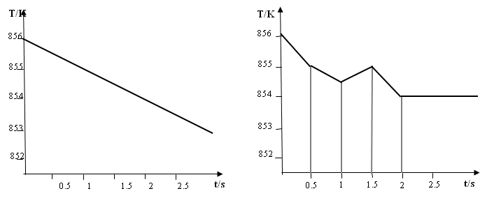
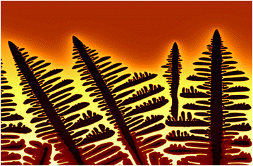
Figure 4
Peritectic dendrites in Fe-C-Mn
Release of latent heat
It is important, if microstructure evolution affects the temperature field. The temperature is calculated by balancing latent heat with net heat extraction. It should be noted that it is not compatible with the moving-frame option. In this case, the heat flux over time shall be specified (Figure 5).
Figure 5
Defining heat flux over time for latent heat release
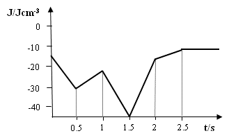
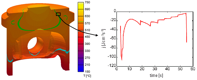
Figure 6 shows a model of an automotive piston where latent heat release has been considered. The material here is a five component aluminium alloy. In the numerical modelling, the homogeneous melt is cooled with a constant heat extraction rate. A seed density model has been applied for nucleation of primary silicon particles. During growth of the primary silicon, the melt is depleted from silicon1.
Figure 6
An example for latent heat release: a five component Al-alloy
Periodic boundary conditions
Using periodic boundary conditions with experimental microstructures is a fundamental problem, because experimental structures are never periodic. In that case, an extra grain boundary is formed all along the domain boundary (see the Grain-Growth examples on the MICRESS® distribution CD). At the beginning, what happens may seem quite strange, but with proceeding grain growth, the result becomes acceptable.
Gradient boundary conditions
Gradient boundary conditions should be used if you do not want to obtain additional interfaces. Both isolating and symmetric boundary conditions lead to interfaces which are perpendicular to the border of the domain and this is bad for grain growth.
Important: Gradient BC should be used only for the phase-field. Using them for the concentration field would not only make no sense from physical point of view, but would also lead to instabilities if interfaces between different phases touch the calculation domain boundary.
Cooling rate and temperature gradient
In the standard case, one can assume a linear temperature profile on the microscopic scale. This is the reason, why a cooling rate and a temperature gradient are specified. The meaning of this assumption is that the temperature gradient at the dendrite tip cannot change; only the temperature can change. The relation between the temperature at the tip and the one at the bottom (considered by the input file) depends only on the distance bottom-tip and the given temperature gradient. For a more precise approximation, the 1d_temp option can be used. It applies an external one-dimensional temperature field. In this case, however, thermal boundary conditions need to be specified.
-
Ingo Steinbach. Phase-field models in materials science. Modelling and Simulation in Materials Science and Engineering, 17(7):073001, jul 2009. doi:10.1088/0965-0393/17/7/073001. ↩