Phase Interactions
In this section the user defines the phase interaction data and the grain boundary properties. Phase interactions can be defined for all pair-wise combinations of the phases which have been included in the Phases section.
In the standard input sequence, the user is requested to specify all phase interaction data in a fixed order, starting with the phase pair 0/1. Phase interactions which are not used are switched off using the keyword no_phase_interaction. No further input is required in this case. The standard input sequence is recommended for less experienced users and for low numbers of phases.
Example 1
No phase interaction between phases 0 and 1 and phase interaction between phase 1 and 1
...
# Phase Interactions
# ==================
#
# 0 (MATRIX)  /  1 (PHASE_1)
# --------------------------
# Simulation of interaction between 0 (MATRIX)  and  1 (PHASE_1) ?
# Options: phase_interaction  no_phase_interaction
#  [ standard | particle_pinning[_temperature] | solute_drag ]
#   | [ no_junction_force | junction_force ]
no_phase_interaction
#
# 1 (PHASE_1)  /  1 (PHASE_1)
# ---------------------------
# Simulation of interaction between 1 (PHASE_1)  and  1 (PHASE_1) ?
# Options: phase_interaction  no_phase_interaction  identical phases nb
#  [ standard | particle_pinning[_temperature] | solute_drag ]
#   | [ no_junction_force | junction_force ]
phase_interaction
...
If the number of phases involved in the simulation is high, the input file may get quite long and unreadable, even if most of the theoretically possible phase interactions are switched off. For this case, a terse mode is available, in which only those phase interactions which are needed can be defined in an arbitrary order. The other interactions are automatically switched off. Input is switching to terse mode if the line for the first phase interaction starts with two integers, corresponding to the numbers of the interacting phases. For technical reasons, the section then has to be finished by the keyword end_phase_interactions, if the terse mode is used.
Example 2
Phase interaction data with phase interaction in terse mode
...
# Phase Interactions
# ==================
#
# 0 (LIQUID)  /  1 (FCC_L12)
# --------------------------
# Simulation of interaction between 0 (LIQUID)  and  1 (FCC_L12) ?
# Options: phase_interaction  no_phase_interaction
#  [ standard | particle_pinning[_temperature] | solute_drag ]
#   | [ redistribution_control ] or [ no_junction_force | junction_force ]
0 1 phase_interaction
...
end_phase_interactions
...
Enabling phase interactions means that one of the phases may grow or shrink on the expense of the other. On the other hand, if a phase interaction is switched off, no movement of the corresponding interfaces is possible.
This also concerns the initialisation of the interface: if such an interface is created via the initial grain setting, the interface will stay sharp even if an initialisation is requested (see here). Nevertheless, in case of concentration coupling, there can be diffusion through switched off interfaces. The partition coefficients which are necessary for diffusion through interfaces are accessed from the other phase interactions using a constant-K approximation. If e.g. interactions are defined for phases 0/1 and 0/2, a simplified description can be derived for the ½ interface. This description is stored for each interface cell in the moment of creation (as initial structure or from moving triple junctions) and kept constant during the further simulation steps.
Important: If too many phase interactions are switched off, no calculation of the missing partition coefficients may be possible!
Switching off phase interactions can greatly reduce the complexity of a simulation, especially if many phases are included. In solidification, e.g., it may be wise to discard all solid-solid interactions, if a continuation of the simulation (with heat treatment etc.) is not intended. In case of solid state reactions, only the interactions of the precipitations with the matrix and not the interactions between different types of precipitates should be included. However it should be noted that the constant-K approximation may be problematic in case of phases with very small solubility ranges for some elements (unless they are defined as stoichiometric). Furthermore, excessively extended inactive interfaces in connection with TQ-coupling may lead to a significant performance drop because of their treatment with local scope (see below)
If two contacting phases have a common stoichiometric component without solubility range (see Concentration Solver - Stoichiometry and more), the interaction between these two phases must be switched off!
When the interaction of one phase with itself is enabled, solid-state interactions between grains of the same phase will be activated. In this case, no chemical driving force is included and the movement will be controlled only by curvature (and by stored energies in case of recrystallisation).
As alternative to phase_interaction and no_phase_interaction, the keyword identical, followed by the phase numbers corresponding to another interaction (two integers), can be used for abbreviation purposes, if a phase interaction with exactly the same parameters has already been defined previously.
Phase Interaction options
The option phase_interaction can be followed by optional keywords which selects special interaction models:
-
standard: this is the default interaction -
particle_pinning: enables a mesoscale model for particle pinning. If this keyword is selected, an effective mobility model is used which includes the pinning effect of not explicitly resolved particles. As further input, a critical pinning force, which can by defined either by a pinning pressure [J/cm^3] or [MPa] (default) or a pinning curvature [\mu m^{-1}], and a minimal mobility will be requested later in this section. -
particle_pinning_temperature: enables the mesoscale particle pinning model with temperature dependent input parameters read from an ASCII file. -
solute_drag: the solute drag model is based on a two-step hysteresis description of the mobility for the free and loaded interface, as a function of the interface velocity. If this model is selected, a critical transition velocity, a transition range (for smooth transition) and a drag factor has to be specified. -
redistribution_control: this keyword activates special models which determine the redistribution behaviour. Currently, models for para-equilibrium, for nple as well as for antitrapping are available. These models are further specified in Phase Diagrams). Note that the keyword is also used to activate the automatic mobility correction in the thin-interface-limit for diffusion controlled phase interactions.
Driving Force options
In the next line, the driving force options have to be specified. Except for the local RX model, where these options have to be specified always, they have to be specified only in the case of interaction between different phases. All DeltaG options have to be written in one line, consisting of concatenated pairs of a keyword and the corresponding value (see Example 3).
The keyword avg is used to define averaging of the driving force across the interface. Averaging prevents spreading of the interface in case a strong concentration gradient causes opposite driving forces on both sides of the interface. The user can specify a value between 0 (no averaging) and 1 (maximum averaging), corresponding to a maximum averaging distance between 0 and the interface thickness \eta. As weights for averaging this distance, the interface gradient \sqrt{\phi_\alpha\phi_\beta} , and the intersection lenght of each interface cell with the gradient direction are used.
Averaging of the driving force helps stabilising the interface in case of diffusion controlled transformations, if the resolution is not high enough (i.e., the diffusion length is not big compared to the interface thickness). The recommended value is 0.5, the default value is 0. Alternatively or in addition, interface stabilisation can be used (see 'interface energy and mobility' below).
The keyword max specifies the maximum driving force allowed (value above which the driving force will be cut-off). This value is useful to shrug off some temporary problems during initial transients or to reduce the impact of numerical fluctuations. The value should be chosen high enough in order not to limit kinetics during normal growth.
Important: If a too small value is chosen for the maximum allowed driving force, the movement of the interface can be drastically slowed down and anisotropy is lost!
The smooth keyword has only effect if averaging is specified: The gradient direction, along which averaging of the driving force is performed, is randomly rotated with the specified maximum value in degrees. Depending on other circumstances, this option may help to reduce the effects of grid anisotropy on the growth morphology. A typical value is 45°, default is 0°.
offset can be used to add an extra driving force offset. It can be used to 'correct' small deviations in thermodynamic databases, to add an implicit curvature, to describe martensite as destabilized ferrite, or just to make an interface move in case of uncoupled phase-field.
Example 3
Phase interaction with driving force averaging, temperature dependent surface energy, constant mobility of the phase boundary and isotropic phase interaction between liquid and solid**
...
# Phase Interactions
# ==================
#
# 0 (LIQUID)  /  1 (FCC_L12)
# --------------------------
# Simulation of interaction between 0 (LIQUID)  and  1 (FCC_L12) ?
# Options: phase_interaction  no_phase_interaction
#  [ standard | particle_pinning[_temperature] | solute_drag ]
#   | [ redistribution_control ] or [ no_junction_force | junction_force ]
0 1 phase_interaction redistribution_control
# 'DeltaG' options:  default
# avg ...[] max ...[J/cm^3] smooth ...[Deg] noise ...[J/cm^3] offset ...[J/cm^3]
avg 0.55 max 100
# Type of interfacial energy definition between 0 (LIQUID) and  1 (FCC_L12) ?
# Options:  constant  temp_dependent
temp_dependent
# File for surface energy coefficient between 0 (LIQUID) and  1 (FCC_L12)?
C:\Desktop\Info.txt
# Type of mobility definition between LIQUID and FCC_L12?
# Options:  constant  temp_dependent  dg_dependent
constant
# Kinetic coefficient mu between LIQUID and FCC_L12 [cm**4/(Js)] ?
...
# Is interaction isotropic?
# Optionen: isotropic  anisotropic [harmonic_expansion]
isotropic
...
Interface Energy and Mobility
The interface energy, which scales the effect of curvature, can be given either as a constant value (keyword constant) or defined as temperature_dependent. Temperature dependent values can be read from an ASCII file where the first column represents temperature and the second the interfacial energy. Linear interpolation with temperature is performed on the tabular data. Interface energies have to be specified in J/cm^2.
As a second optional parameter in the same line with the interface energy, a numerical interface stabilisation can be specified as extra value with the same dimensions as the interface energy (J/cm^2). It should have a value which is higher than, but not more than ~10x the interface energy.
One of the most important phase interaction parameter is the interface mobility which defines the interface velocity for a given driving force or curvature. The mobility may be defined as constant, temperature dependent or driving force dependent. In the both latter cases, the user will be asked to provide the name of a text file where the kinetic coefficient (second column) is given in tabulated form as a function of temperature or driving force (first column). Otherwise, just a constant value in cm^4/Js is required. In case of some special models (solute drag, particle pinning), additional model parameters have to be included here (see above). As second optional parameter a minimum mobility can be defined which limits reduction of the mobility by automatic time stepping (minimal time step), anisotropy or special models like particle pinning. If the interface motion is controlled by solute diffusion, it is generally required to correct the effect of the finite interfacial width. This can either be done manually by calibration or automatically by selecting the keyword phase-interaction with the option redistribution-control and the further specification mob_corr in the phase-diagram section. Note that in case of complete diffusion-control, the exact value of the kinetic coefficients does not play any role, but has to be defined high enough not to slow down the interface motion.
Misorientation
The crystallographic interaction of two anisotropic phases is split into two factors: first, the misorientation function which considers the grain orientations relative to each other and second, the anisotropy function which considers the relative orientation of the boundary plane (given by the interface normal vector). If the keyword misorientation is set, the reduction of the mobility and the interfacial energy can be specified as function of the misorientation angle or by a constant factor (see Example 4). Note that the misorientation model accounts for the defined crystallographic phase symmetry and always calculates the lowest misorientation angle from all equivalent rotations. The keyword low_angle_limit allows specification of the transition angle (in degree) between low angle and high angle boundaries. Per default, this angle is set to 15°. The additional option special_orient allows definition of special misorientation relations, such as twin and twist boundaries. It can be used in combination with the keyword aniso_special_orient (instead of anisotropic) to define an anisotropy function which only applies to interface with a special orientation relation, while all other interfaces are treated as isotropic.
The reduction of the interfacial energy as function of the misorientation angle \theta is governed by the implemented Read-Shockley law1:
where \gamma_{HAB} and \theta_{HAB} are the interfacial energy of high angle grain boundary, specified above, and of the transition angle respectively.
The function is depicted in Fig.3.8. Note that for misorientation angles below 0.5°, \gamma(\theta) = 0.1 \gamma_{HAB}.
Figure 1
Reduction of the interfacial energy and mobility as function of the misorientation angle between two cubic grains.
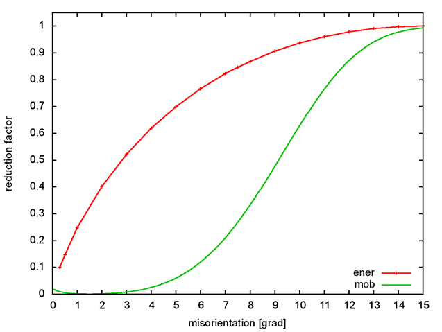
The reduction of the interfacial mobility as function of the misorientation angle between cubic grains is described by the sigmoidal law suggested by Humphreys[@Humphreys1997] (see Figure 1):
where m_{HAB} is the interfacial mobility of a high angle grain boundary. B and n are two model parameters, which can be fitted if experimental data are available: Per default, B=5 and n=4. In order to avoid small mobilities at very small misorientation angles, the Humphreys law is cut below 1.5°:
Example 4
Reduction of the surface energy and of the mobility of a low angle misorientation between cubic grains, according to the Read-Shockley and Humphreys model respectively.
...
# Phase interaction data
# ==================
#
# 1 (PHASE_1)  /  1 (PHASE_1)
# ---------------------------
# Simulation of interaction between 1 (PHASE_1)  and  1 (PHASE_1) ?
# Options: phase_interaction  no_phase_interaction  identical phases nb
#  [ standard | particle_pinning[_temperature] | solute_drag ]
#   | [ no_junction_force | junction_force ]
phase_interaction
...
# Shall misorientation be considered?
# Options:   misorientation    no_misorientation
#           [low_angle_limit <degrees (default=15)>]  [special_orient <nb>]
misorientation low_angle_limit 15
# Input of the misorientation coefficients:
# Modification of interfacial energy for low angle boundaries
# Options:  factor   read-shockley
Read-Shockley
# Modification of the mobility for low angle boundaries
# Options: {factor | humphreys [<minimum> <parameter B> <parameter N>]}
#                    (default: minimum=0. B=5.0 N=4.0)
humphreys 0.01 5.0 4.0
...
Anisotropy
If at least one of the two interacting phases has been defined as not isotropic, the pairwise interfacial properties may be defined as anisotropic, i.e. as function of the local interface normal. Two alternative model versions can be chosen to describe weak non-faceted anisotropy: The default standard model offers predefined anisotropy functions. The specific choice of the anisotropy function depends on the crystal symmetry of the anisotropic phase, previously defined by the user. The user can specify anisotropy coefficients \delta_{\sigma*} and \delta_{\mu} in the range of \delta \in [0,1]. A typical value for \delta_{\mu} in cubic metal systems is 0.05. The more complex harmonic_expansion model allows to formulation of anisotropy functions by combination of spherical harmonics in accordance with the selected crystal symmetry. The implemented harmonic functions are listed in Table 4 of Topics:Phase Interaction. In case of faceted anisotropy, individual sets of anisotropy coefficients \delta_{\sigma*} and \delta_{\mu} can be defined for each facet type. Note that the value 1 here corresponds to isotropic growth and the strength of anisotropy increases with decreasing coefficient, see Topics/Phase Interaction/Faceted anisotropy.
Phase Diagram
An enabled phase interaction requires a phase diagram if the phases are not identical.
In case of uncoupled or temperature coupled simulations (phase or temperature in the Model section), the pair-wise thermodynamic data are described only by the equilibrium temperature and the entropy of fusion (see Example 5). For concentration coupling, however, thermodynamic data are much more complex. The rest of this chapter deals with this case.
Example 5
Definition of equilibrium temperature and entropy of fusion
...
# Phase Interactions
# ==================
# 0 (MATRIX)  /  1 (PHASE_1)
# --------------------------
phase_interaction
...
# Equilibrium temperature between MATRIX and PHASE_1 ? [K]
800.00
# Entropy of fusion between MATRIX and PHASE_1 ? [J/(cm**3 K)]
0.50000
...
If Thermo-Calc™ coupling (via its TQ interface) is NOT to be used, the user has to provide a linear phase diagram description. There are two formats which can be selected, either linear or linearTQ. The first corresponds to the normal linear description which consists of the temperature at the reference point, the entropy of fusion, and the reference concentrations and slopes for all elements in both phases. The matrix component is omitted in this description.
Example 6
Phase diagram input data with no coupling to a thermodynamic database
...
# Which phase diagram is to be used?
# Options:       linear        linearTQ
linear
# Temperature of reference point? [K]
350.0000
# Entropy of fusion between MATRIX and PHASE_1 ? [J/(cm**3 K)]
0.8
# Input of the concentrations at reference points
# Reference point 1: Concentration of component Comp_1 in phase MATRIX ? [at%]
10.
# Reference point 2: Concentration of component Comp_1 in phase PHASE_1 ? [at%]
5.000
# Input of the slopes at reference points
# Slope m = dT/dC at reference point 1, component Comp_1 ? [K/at%]
-4.000000
# Slope m = dT/dC at reference point 2, component Comp_1 ? [K/at%]
-8.0000
...
The second format is identical to the internal extrapolation which MICRESS® uses in case of Thermo-Calc™ coupling, and thus exactly corresponds to the output format of initial linearisations in the .log output file. In addition to the normal linearisation parameters (keyword linear), this format includes a driving force at the reference point and an explicit temperature dependence of the reference concentration. Moreover, the transformation entropy is replaced by the temperature derivatives of the driving force with fixed composition in phase 1 or phase 2 (dSf+, dSf-).The advantage of the linearTQ input format is that linearisation parameter obtained in Thermo-Calc™ coupled simulations (found in the .log or .TabLin output file) can directly be used as linear phase diagram description in a subsequent simulation. Another important application is the use for eutectic systems with solid-solid phase interactions: The slopes of the phase diagram lines for the interaction of the two solid eutectic phases typically have opposite signs. This reflects their immiscibility which is enhanced with lowering temperature. This however is not a demixing effect and can be correctly treated by using the linearTQ phase diagram description with different signs for, dSf+ and dSf.
Note: The .log output of the initial linearisation parameters for a phase interaction additionally contains information on the transformation enthalpy which is not part of the phase diagram description. For sake of simplicity, during input of the linearisation parameters in the linearTQ format, a dummy variable is read for the enthalpy. Thus, the output block in the .log file can be directly transferred to the driving file by copy and paste without removing the transformation enthalpy. If data are taken from other sources (e.g. the .TabLin file), a dummy value has to be included in the corresponding place.
A phase diagram description in the linearTQ format can NOT be exactly translated into a normal linear phase diagram description. If in a linearTQ phase diagram description dSf+ and dSf- have opposite sign, the slopes of ALL elements in the two phases must also have opposite signs.
Next, the thermodynamic description of the phase interaction has to be given: for each interaction, data can be taken from the specified database, from a linearised description (linear) or according to the linearTQ format (see above).
In case of database, an optional keyword in the same line with database can be used to specify the scope or region, in which the input parameters to the quasi-equilibrium calculation are averaged (T, c, \phi) and for which the calculated linearisation parameters are valid. In case of local, each interface cell which exists for the given phase interaction bears its own local linearized description obtained and updated from the database according to the specified updating conditions. Averaging of input parameters is done only along the interface gradient if avg has been specified in the 'dG-Options'.
Otherwise, only one description is obtained and updated for each reference scope. The non-local option are generally less accurate, especially if the corresponding regions are spatially extended. In turn, they are computationally much more efficient and furthermore reduce numerical noise. The non-local options are:
-
interface: Each interface between two specific grains will get its own data set, which strongly reduces the effort of updating. This scope comes with a low administrative overhead, but suffers from inconsistencies at triple junctions, which may lead to spurious triple point movements (which are independent from the updating interval). -
interface_fragment: Similar tointerface, but increased 'locality' and exactness by narrowing the spatial scope to each interconnected segment ('fragment') of the interface region for a specific grain pair. -
global: Uses one set of linearisation data for all interfaces between two phases, so that it comes close to a linearized phase diagram where the data are automatically calculated and updated based on the average interface composition and temperature. This mode can be regarded as a fully global description. -
fragment: Defines common linearisation data for interconnected segments ('fragments') of all phase interfaces which thus may span several grain interfaces belonging to the same phase pair.
In terms of 'locality', the following order can be tentatively defined:
local > interface_fragment > interface > fragment > global
All non-local options can further be restricted by definition of a distance parameter (half diameter) which intersects each spatial scope into separated regions. Although coming with some computational overhead, this allows adapting to your specific needs, thus allowing the user to optimize exactness vs. computational performance, especially in case of strong temperature gradients and correspondingly high temperature differences in the simulation domain. The distance (in µm) is written directly after the scope keyword in the same line (see Example 7).
For all non-local linearisation scopes, in multi-phase regions (triple junctions) the reference regions for the linearisation parameters of the coexisting phase interactions typically do not match. This may lead to local inconsistencies between the different phase interfaces, because they use linearisation data sets which may be based on concentration averages on different spatial regions (as the integration area at the same time includes dual interface regions). If necessary, this problem can be avoided using the option database_consistent (see Numerical Parameters for Concentration Solver) which further separates the triple point areas from the dual interface regions both in terms of the range of averaging of interface compositions as in terms of the range of validity of the linearisation data.
After defining the phase diagram input for each phase interaction, in case of Thermo-Calc coupling the updating mode (relinearisation interval) must be specified. While none skips this option, an additional updating time interval can be specified for each phase interaction using the keyword manual or reading the interval time-dependent from file using from_file (see Example 7). Setting a high value for the updating interval speeds up the calculation by limiting the number of calls to the TQ-library, but at the expense of precision. If the updating interval is specified using the manual option, a temperature interval can be specified by putting the minimum and maximum temperature in the same line. Then, above the maximum temperature and below the minimum temperature no extra updating will be done for this phase interaction. Alternatively, a critical local temperature deviation for updating the thermodynamic description can be specified using the option automatic. This option automatically adjusts the updating interval to the cooling conditions, but does not work for isothermal simulations. Generally, the definition of a relinearisation mode per interface can be helpful, if one phase interaction, e.g. for a specific intermetallic phase, needs more care.
Important: Updating the linearized phase diagram description for each cell or region (depending on scope) is essential for maintaining thermodynamical exactness, especially if temperature or local compositions have changed.
Note: A relinearisation condition for all phase interactions already has been defined in Section Database. Furthermore, MICRESS automatically performs updates for any scope region of moving interfaces: As soon as the share of new interface cells which have been created by movement since the latest update exceeds 50% of the total number of cells of this region, an update is triggered for this region. There is no extra screen output, but the total number of such updates is indicated in summarized form on screen at each output time step.
Further Useful Information: The extent of the individual regions with common linearisation data may change rapidly with time due to moving interfaces and user-defined updating schemes. The regions can be visualized using the .numR output (see Output, where a common reference number indicates that a common set of linearisation parameters was referenced at output time. Using this reference number, the corresponding linearisation parameters can be found in the .TabLin output text file (under 'Alternative Listing').
Example 7
Specifying relinearisation option for an interface
...
#
# 0 (LIQUID)  /  1 (FCC_L12)
# --------------------------
# Simulation of interaction between 0 (LIQUID)  and  1 (FCC_L12) ?
...
# Which phase diagram is to be used?
# Options: database [local|global|interface|fragment][<maximal distance>]
#          | linear | linearTQ
database global 0.5
# Relinearisation interval for interface LIQUID / FCC_L12
# Options:  automatic   manual   from_file   none
manual 0.001 900. 1100.
#
# 0 (LIQUID)  /  2 (FCC_L12#3)
# ----------------------------
# Simulation of interaction between 0 (LIQUID)  and  2 (FCC_L12#3) ?
...
# Which phase diagram is to be used?
# Options: database [local|global|interface|fragment][<maximal distance>]
#          | linear | linearTQ
database fragment
# Relinearisation interval for interface LIQUID / FCC_L12#3
# Options:  automatic   manual   from_file   none
from_file
# File name for the time-dependent relinearisation interval
relinInterval0_1
...
Redistribution Models
If redistribution_control has been defined (at the beginning of the input data for the current phase interaction), further specification of the Redistribution Model is required for each element. The following options are available:
-
normal: Normal redistribution according to the extrapolation scheme chosen in Numerical Parameters for Concentration Solver is applied for the given element. -
nple: Redistribution is calculated according to thenplemodel. With this model, the total composition, which is used as an input to thenormalredistribution model, is shifted in such a way that the phase compositions of the whole interface adopt the equilibrium compositions of a stationary front. The moving direction of the interface can either be determined by the local velocity, the average velocity of the interface, or the rate of the bottom temperature (see below). The most typical application example are solid-solid phase transformations in steels, where diffusion of interstitial elements determines the phase transformation rate, while substitutional elements are redistributed without diffusion (i.e. their diffusion pile-up is much shorter than the numerical interface thickness). -
para: Redistribution is calculated according to theparapara-equilibrium model. This is similar to thenpleoption. However, with this model the total composition is shifted in such a way that the contribution of the substitutional elements to the driving force vanishes. Like thenplemodel, theparamodel calculates the phase compositions depending on the moving direction of the interface. -
paratq: Redistribution is calculated according to theparatqpara-equilibrium model. This model applies the para-equilibrium condition already during calculation of quasi-equilibrium, while the redistribution itself is performed like for thenormaloption. This keyword can only be used if TQ-coupling is performed. -
atc: Redistribution is calculated in a way which corrects for numerical trapping effects of the diffuse interface ('anti-trapping'). This is achieved by an additional diffusion flux along the interface gradient2. Please note thatatcrelies on values of the diffusion coefficients of both phases which per default are averaged over the interface region. Different averaging scopes can be applied using the 'tic-options' in Numerical Parameters for Concentration Solver.
In case of normal or atc, the additional keyword mob_corr can be given in order to activate a mobility correction, which can be adjusted by a further prefactor (<1 for increasing the calculated interface mobility).
In case of nple or para, separate redistribution models can be defined for the forward and backward direction of motion if two options are specified in the same line.
In case that any of the keywords nple or para has been used in any of the phase interaction, an extra input of the reference for the moving direction of the interfaces has to be specified at the end of Section 'Phase Interactions'. The options are:
local_velocity|average_velocity|bottom_temperature
Although the use of local_velocity would appear most logical, numerical noise in the interface velocity can lead to serious problems. Therefore, bottom_temperature should be chosen whenever the transformation direction is expected to be in accordance with the temperature rate applied at the bottom.
References
-
Janin Eiken. A Phase-Field Model for Technical Alloy Solidification. RWTH Aachen University, 2009. ISBN 9783832290108. ↩
-
A. Carré, and B. Böttger, and M. Apel. Implementation of an antitrapping current for a multicomponent multiphase-field approach. Journal of Crystal Growth, 380:5–13, 2013. doi:10.1016/j.jcrysgro.2013.05.032. ↩