Numerical Parameters
In this section, some purely numerical parameters for the phase-field, concentration, flow and stress solver are defined.
Phase-Field Solver
Time stepping
The time step for the phase-field solver has to be defined. It is recommended to use the automatic or automatic_limited time step options. In the latter case, minimum and maximum values for the time step as well as optional correction factors (default 0.9) can be further specified which apply to the "phase-field" and "segregation" time stepping criteria. Not all of the 4 parameters must be given. Especially, the first value, the minimum time step, can be very useful to improve performance (for more details please use the MICRESS® forum at www.micress.de). The parameters for automatic_limited can also be read as time-dependent from a file.
For manual definition of the phase-field time step, only the corresponding value in seconds has to be given. As a hint for finding reasonable values, the time-steps for each phase pair according to the automatic criteria is given as screen output during initialization (see Figure 1.
The section ends with the definition of the number of iterations for initialisation of the interfaces. During these types of iterations, the sharp interfaces produced by the initial grain structure setting are smoothed by applying the phase-field solver without any chemical driving force. Due to the fact that the stabilisation term, which enforces the interface profile, and the curvature are not separated in the phase-field model, curved initial grains will shrink and finally vanish if the number of iterations is too high. For single round particles, an attempt has been made to compensate for that, but in the general case this cannot be avoided. In most cases, there will be no problem, if a small number (ca. 20) of initial iterations is used. On the other hand, the non-conserved phase-field variable gives the opportunity to fine-tune the initial grain fraction during initialisation, e.g. if the "sharp" grain consists of only a few grid cells.
Example 1
(Limited) Automatic time stepping with 10 iterations for initialisation
...
# Phase field solver
# ------------------
# Time-step ?
# Options:   fix ...[s]   automatic    automatic_limited
automatic_limited
# Options:   constant      from_file
constant
# Limits: (real) min./s, [max./s], [time step factor], [segregation factor]
1.E-6 1.E-2
#Coefficient for phase-field criterion 1.00
#Coefficient for segregation criterion 0.900
# Number of steps to adjust profiles of initially sharp interfaces [exclude_inactive]?
10
...
Figure 1
Screen output for time step initialisation
...
Beginning of initialisation
===========================
...
Routine init calls routine initTwidth

tWidth_max( LIQUID: FCC_A1) = 2.0552885E-05 s
tWidth_max( LIQUID: ALCU_THETA) = 1.0687500E-05 s
Maximal value for tWidth = 1.0687500E-05 s for phase-field solver
Maximal value for tWidth = 1.0687500E-06 s for conc-field solver
Automatic time stepping (phase-field solver): decreased value for tWidth = 1.01531E-06 s
Initial value for tWidth = 1.01531E-06 s for automatic time stepping (phase-field solver)
...
Type of potential and FD-correction
The user can select either double_obstacle or multi_obstacle.
The double_obstacle functional is of parabolic type: g(\phi)=\phi(1-\phi), limited by discontinuities at \phi=0 and \phi=1. The multi_obstacle functiona 1 represents its generalized formulation for multiphase systems comprising contributions g_{\alpha\beta}(\phi)=\phi_\alpha \phi_\beta for all pairwise phase interactions. In the special case of a two phase systems, it exactly recovers the double_obstacle functional. We recommend to use multi_obstacle as a standard for all applications.
If double_obstacle is selected for simulation of a multiphase problem, the anti-symmetric approximation1 will be used. In this simplifying treatment, pairwise interactions between phases \alpha and \beta are directly derived from the corresponding two phase free energy functionals f_{\alpha\beta} instead of from the common free energy functional, thus neglecting higher order contributions \alpha\beta\gamma. As a consequence all dihedral angles at a junction will evolve as equal (i.e. a triple junction in 2-D will always exhibit three 120° angles) independent of the energies of the adjacent interfaces. Therefore, this approximation can only be used in cases in which all boundaries energies are equal or in which dihedral angles are of no importance. For a correct reproduction of dihedral angles in multiphase problems select multi_obstacle. Keep in mind that strongly differing interfacial energies may lead to high junction forces and extreme angles.
The numerical solution of the phase-field equation based on finite differences (FD) inherently implies a discretization error which may strongly bias the simulation results. Usually, it results in too low interface velocities. The error is inversely correlated to the number of numerical cells resolving the diffuse interface profile. However, high numbers of interface cells are detrimental for computational performance and also favor undesired numerical interface trapping. The problem can be overcome by an improved numerical solution of the phase-field equation, which takes advantage of the a priori knowledge of the phase-field profile, determined by the choice of the potential function2 3. To activate this improved numerical solution, select fd_correction and choose an interface width of 3-4 numerical cells. If you want to rerun a diffusion-controlled simulation which has been run before without the fd_correction option, it might be necessary to recalibrate the interface mobility. The option fd_correction is recommended to be used as a standard for all applications and may become default in coming versions. It is however not yet compatible with temperature coupling.
The option multi_obstacle especially comprises corrections for triple junction terms and is important for correct wetting characteristics.
Phase Minimum and Interface Thickness
Next, a value for the phase minimum is required. A cell with a phase or grain fraction below this value is not considered to be in the interface any more but in a bulk region (liquid or solid). In most cases, a value of 1.E-4 can be recommended.
As optional parameter in the same line, a hysteresis factor can be defined which has a default value of 2, For more information, please consult the MICRESS® forum.
The interface thickness (in cells) also has to be input in this section. Generally, with increasing interface thickness, the curvature evaluation of the phase-field profile is improved. On the other hand, a higher resolution is required to resolve highly curved structures, and numerical artefacts related to the finite interface thickness like artificial solute trapping" is increased.
Note that in case of using extremely small values for the interface thickness (less than 3 cells), curvature evaluation is poor and nucleation at the interface is not working correctly anymore!
Phase-Field Data Structure
In this section, the initial dimensions for the internal fields iFace and nTupel must be specified. During runtime, the size of these fields is determined automatically, so in most cases the given values are of minor importance
The values have to be given relative to the size of the simulation domain, a value of 1.0 for iFace for example would assume that the whole calculation domain could be covered by (two-grain or two-phase) interfaces without exceeding the given initial list size. The same holds for nTupel and the coverage of the domain with triple or higher junctions. The actual usage for both fields can be found in the TabL output.
The arrays iFace and nTupel are fully dynamic, so the influence of the initial values is quite limited. In extreme cases, the specification of excessively high initial values can lead to a memory overflow during the program startup. Too low values can lead to an unnecessarily high number of reallocation steps which slow down the initialisation process e. g. in the case of grain growth simulation with a high number of initial grains. Initial values of 0.1 for both parameters are recommended and work in practically all cases.
Additional optional parameters can be specified for the minimal and the target usage. These parameters allow a fine-tuning of the reallocation criteria during runtime what can be helpful if a temporal memory overflow must be avoided. More details can be found or requested in the MICRESS® forum.
Example 2
iFace and nTupel
...
# Phase field solver
# ------------------
...
# Coefficient for initial dimension of field iFace
#  [minimum usage] [target usage]
0.10
# Coefficient for initial dimension of field nTupel
#  [minimum usage] [target usage]
0.10
...
Concentration Solver
The maximum number of concentration solving per phase-field iteration has only to be defined, if concentration coupling is used in combination with a fixed phase-field time step. An error message is given if the number is too small to be consistent with the time-step criterion of the explicit diffusion solver. This input is not required when automatic time-stepping is used.
The global cushion factor influences the diffusion time stepping, i.e. the lower the factor the smaller are the diffusion time steps. In MICRESS version lower than 7.0, this factor holds a default value of 0.5 to be on the safe side. However, reducing the diffusion time stepping by 5% is sufficient for the most applications and gives a performance boost for the diffusion solver part.
Example 3
Diffusion time stepping factor (cushion)
...
# Concentration solver
# --------------------
# Factor for diffusion time stepping?  (0.0 < factor < 1.0)
0.95000
...
Stoichiometry and more
This section of input represents a terse loop with different leading keywords which can be placed in any order and must be closed by the keyword end_of_options. In case of multiple definitions, the last input will overwrite previous definitions. Besides the highly relevant definitions of stoichiometric conditions and a diagonal extrapolation scheme, the options are mostly very specific and only needed in special cases. Nevertheless, it is important to have them for those cases. A list of these options appears in the cleaned-up version of the input file to remind the users about their syntax:
Figure 2
Screen output for Stoichiometry and more
...
# Optional parameters for thermodynamic definitions
# Finish input with 'end_of_options'.
#   {stoichiometric | stoich_solubility | stoich_enhanced} <phase> <component list>
#   steep_limit <value>
#   limits <phase> <component> <min (at%)> <max (at%)>
#   penalty <phase> <phase 2> <component>
#   interstitial <phase> <component list>
#   sum_limits <phase> <component list> <min (at%)> <max (at%)>
#   diagonal [<component list>]
#   interaction <component 1> <component 2>
#   {criterion_higher | criterion_lower} <phase> <phase 2> <component>
#   {ordered | disordered} <phase> <sublattice 1> <sublattice 2>
#   switch_diff_data <phase> <reference phase>
#   {diff_comp_sets | vol_comp_sets | enth_comp_sets} <phase list>
#   temp_limit_TQ <lowest (K)> <highest (K)>
#   temp_limit_phase_TQ <phase> <lowest (K)> <highest (K)>
#   independent_sublattice <phase> <submatrix component> <component list>
#   database_consistent
#   pressure <value (MPa)>
#   start_value <phase> <phase 2>
#   init_fraction <phase> <phase 2> <fraction>
#   tic_tq_segments | tic_z_segments
...
The individual options often have complex applications and effects and will be described only briefly here. For more details please consult the MICRESS Forum or use the MICRESS Support (support@micress.de).
-
stoichiometric|stoich_solubility|stoich_enhanced: The first type of required information is a list of all the stoichiometric components, which can be defined using the keywordstoichiometricfollowed by a phase number and a list of element numbers. Stoichiometric components are those elements in a phase for which no explicit slopes of the phase diagram lines are specified or can be specified. A typical case is an element which has no solubility range in a given phase (line compound), which also includes elements with zero solubility. In such cases, the composition of the element in this phase cannot be used as a thermodynamic condition, which is important information if coupling to thermodynamic data is used. This type of stoichiometric condition is automatically detected and needs not to be (but may be) specified by the user.
The user may also decide to define an element with large slope in the phase diagram for numerical reasons as stoichiometric, other reasons could be opposite signs of the solidus and solvus slopes retrieved from the database, which also can create numerical problems (pseudo-binary "demixing").
Contrarily, the keywordsstoich_solubilityandstoich_enhancedare expert options which should not be used without prior consultation of MICRESS® experts. The first one can be used to indicate that the addressed element has a solubility range and thus its composition can be used as a thermodynamic condition when calculating quasi-equilibrium or phase properties like diffusion coefficients or enthalpies. However, redistribution will be performed with a stoichiometric condition, e.g. because multi-binary demixing would be expected. The second option (stoich_enhanced) presents a more effective extrapolation scheme for redistribution, which assumes a "solidification path" approximation similar as in the growth restriction theory for nucleation. Although this approximation is not necessarily correct, it can be better than just assuming a constant composition, especially during solidification. It automatically implies alsostoich_solubility. -
steep_limit: When an element in a phase is defined as stoichiometric with solubility range (stoich_solubility), MICRESS® will not only use concentration conditions for thermodynamic calculations, but also try to calculate the slopes during initialisation of the phase interactions of this phase. If the slopes of the interacting phases differ by more than a factor of 1.0*10^5, is is preferred not to calculate this slope again during the further simulation run. This has not only effects on solute redistribution but also for the dS+ and dS- value (see Phase Diagram). The optionsteep_limitallows specifying a different value for the critical factor. -
limits: This option is followed by a phase and component number in the same line and restricts the allowed composition range of an element in a phase. The minimum and maximum value in at% (always!) is specified in the same line, or alternatively as two extra lines. In case of TC-coupling, MICRESS during initialisation tries to calculate theoretical limits based on the sublattice constituents defined in the thermodynamic database. If compositions outside of this range were used as conditions in Thermo-Calc calculations, serious errors would occur. For this reason, knowledge of these limits is crucial. In case of full solubility of all elements or VA constituents in all sublattices, a minimum of 0 at% and a maximum of 100 at% are obtained as default limits.
The role of thelimitsthus is to restrict allowed composition ranges for TC-coupling (by raising a TQ-error with number "1xxyy" with xx=phase, yy=component), but also (in connection with the optionpenalty) to prevent crossing these limits as a result of a too far extrapolation of linearisation data (leading e.g. to negative compositions).
User-definedlimitsare especially helpful if the same phase in the database exists as several composition sets (e.g. FCC_A1 and FCC_A1#2), andswitchingbetween the two phases has to be avoided. -
penalty: With this option apenaltydriving force is triggered if an element in the specified phase and phase interaction crosses its default or user-defined limits. This helps to avoid conditions which lead to compositions outside the user limit. As penalty term can sometimes lead to strange side effects (especially when several competing limits take action), this option should be used carefully and only if necessary. -
interstitial: If thevolume_changemode is activated, components can in this section be defined asinterstitialby using this keyword followed by a phase number and component number(s). By default, components are defined as substitutional, if no 'VA' constituent is present, and as interstitial otherwise. In contrast to substitutional diffusion, diffusion of interstitial components is related to a local change in number of moles.
Besides thevolume_changemode, interstitial elements also affect quasi-equilibrium calculation and the eigenstrains from database in case of stress coupling. -
sum_limits: Similar tolimits,sum_limitstrigger TQ-errors ("1xx99" with xx=phase) if the sum of the concentrations of a given set of elements falls below or exceeds a user-defined limit (e.g. to prevent switching between \gamma and \gamma'-phase in Ni-alloys. In contrary tolimits, no defaultsum_limitsare defined. Only onesum_limitsoption can be defined per phase, and - for conceptual reasons - no correspondingpenaltyoption exists. -
diagonal: Switches for the list of elements from 'Multi-binary Extrapolation' to 'Diagonal Extrapolation'42
The use of stoichiometric conditions, especially when applied to avoid pseudo-binary "demixing", can easily come to a limit: It is generally not recommended to set a stoichiometric condition for the same element in two phases between which a phase interaction is defined (see section Phase Interactions). With this limitation it may be almost impossible to avoid the effects of pseudo-binary "demixing" in materials like stainless steels by use of the stoichiometric condition.
Therefore, from MICRESS® version 6.1, a 'Diagonal Extrapolation Scheme' has been included which only uses the diagonal elements of the redistribution matrix and which avoids demixing at the costs of a slightly lower extrapolation accuracy (which can be compensated for by more frequent updating of quasi-equilibrium).4 It is invoked by specifying the keyworddiagonal, followed by a list of elements. Ifdiagonalis used without further parameters, this extrapolation is applied for all dissolved components. -
interaction: Switches to 'Ternary Extrapolation' of the two specified elements and the matrix component.
'Ternary element interactions' can be included for selected element triples. Ternary extrapolation gives the user the possibility to account for some of the interactions between the (dissolved) elements which are neglected in case of normal (pseudo-binary or diagonal) extrapolation, and thus to increase extrapolation accuracy. Usinginteractionfollowed by two component numbers in the same line, a ternary interaction group can be established between two elements and the matrix component. Depending on the total component number, several such ternary interaction groups can be defined in extra lines, but each (dissolved) component can be used only once. The definition of ternary interaction groups applies to all phases and phase interactions.
If one of the keywordsinteractionordiagonalhas been used, two partition matrices per phase interaction (one for each direction) are written to the .log file (together with the linearization data, at the time of initialization of the phase interaction) which allow estimating the level of chemical higher order interactions between the dissolved elements and can serve as a guide for usinginteractionin an efficient way. More information about the different extrapolation schemes available in MICRESS® can be found in 4. -
criterion_higher/criterion_lower: These options can be regarded as alternatives forlimitsas they allow for setting a relative limit to phase compositions. The keyword is followed by three integer values for phase 1, phase 2 and a component number. The options allow the user to require that the specified component has a higher or lower composition in phase 1 than in phase 2, otherwise a TQ-error with number "1xxyyzz" (xx:phase1, yy:phase2, zz:component) is raised. This option is helpful e.g. for the interaction of γ and γ' in Ni-base superalloys to ensure that e.g. the Al composition is always lower in γ than in γ' without necessity to specify a discrete composition limit. -
ordered/disordered: If an order-disorder transition is implemented in the sublattice model of a phase in the database, the site fractions of two sublattices are either different (ordered) or identical (disordered). Using these options for a given phase and the specified sublattices (usually no. 1 and 2) checks whether the required condition is violated and creates a corresponding TQ-error ("4xx00" with xx=phase number). -
switch_diff_data: Allows using diffusion data from a different phase. This may be helpful for using the same data also for composition sets, or use diffusion data from a similar phase if for the given phase no data are available. -
diff_comp_sets/vol_com_sets/enth_comp_sets: Allows adding composition sets to single-phase equilibrium calculations which are necessary when retrieving diffusion, volume or enthalpy data. Each keyword is followed by a phase list for which existing composition sets (those with the same base name) are added. Only those composition sets are added which are defined as extra phases in MICRESS® and which already have been initialized. The option helps to deal with problems when working close to miscibility gaps so that the phase at the average composition may be unstable. -
temp_limit_TQ: In case of TQ-coupling, the use of temperatures for any type of TQ-calculation can be restricted to a user-specified range. The purpose of this option is to avoid numerical problems with too high or too low temperatures, which often are an issue in connection with additive processes at full-scale. -
temp_limit_phase_TQ: Identical to temp_limit_TQ, but only for a given critical phase and its phase interactions (e.g. \gamma' at low temperatures). -
independent_sublattice: This is an experimental option which tries to treat the sum rule of an independent sublattice (with loss of a concentration condition) -
database_consistent: affects the scopes of relinearisation options (see Phase Diagram). -
pressure: Allows using a different value than 1 atm as system pressure (especially relevant in case of gas reactions). -
start_value: Allows controlling which of the phase compositions is used as start value for the iteration of the quasi-equilibrium. As parameters, the chosen phase and the second phase of the interface must be given. Default is the use of the phase with higher fraction if no stoichiometric conditions are set. This option has to be considered as an absolute 'expert option'. -
init_fraction: Allows controlling the phase fraction of the specified phase for initialisation of its interface with a second phase. Failing of the initial equilibrium must be avoided at any cost. This option is an alternative or addition to the selection of a suitable temperature for initial equilibrium. Initialisation is performed either at the beginning of the simulation, or when nucleation for a phase, which would establish this interaction, is checked first time (then the temperature for initialisation would not apply anymore). The initial set of linearization data is written in the .log output.
Without this option, a fraction of phMin is used for nucleating phases, or 0.5 for phases already existing in the initial microstructure. After the keywordinit_fraction, the phase itself, the second phase in the interface, and the initial fraction of the phase are specified. -
tic_tq_segments|tic_z_segments: For reasons of computational performance and numerical stability, the thin interface correction models for 'quantitatve phase-field' ('tic-models')atcandmob_corr(see Redistribution Models) refer to averaged values for the thermodynamic linearisation data, temperature, and diffusion coefficients. Per default, the averaging scope is 'per interface'. With the two optionstic_tq_segmentsandtic_z_segments, the scope can be further narrowed down by intersection with either the TQ-segments (as defined by the scopes for relinearisation, see Phase Diagram) or with the z-segments used for calculation of diffusion coefficients (see Diffusion).
Example 4
Expert options for thermodynamic definitions
...
# Concentration solver
# --------------------
...
diagonal
stoichiometric 2 1 2
stoichiometric 3 1-3
limits 0 1 0. 20.
disordered 1 1 2
tic_tq_segments
temp_limit_TQ 973 2000
no_more_options
...
Volume-Expansion Solver
In case that the volume_change has been specified, tow values have to be specified which control the expansion-relaxation solver: first, the maximal number of and second, a convergence value. The task of the expansion-relaxation solver is to homogenize local expansion by compensating material fluxes. The solver runs iteratively and stops when either the specified number of calls per times step is reached or when the mean difference in local expansion falls below the specified convergence value. The effectivity of the solver can be checked by monitoring the degree of homogenization in the expansion output file expa and the consumed CPU-time listed in the TabP file (row: expansion time).
Temperature Solver
If 1d_temp has been specified in Model - Thermal Conditions, a reference position for the .dTLat output is required which lies inside the MICRESS domain (1 < z < CellsZ). The .dTLat output will summarize data on enthalpies and latent heat for that part of the microstructure domain, which belongs to the same grid cell of the 1d-temperature field as the specified z-location.
The keyword 3d_correction switches on a correction of the amount of latent heat which may be wrongly predicted in some types of 2D simulations. An additional phase number input allows specifying a reference phase for this correction, otherwise phase 0 is assumed. If lat_heat_3d is chosen, the user can activate or deactivate the 2D/3D correction for each further phase by the keywords pseudo_3D / no_pseudo_3D followed by the critical fraction of the matrix phase for limiting the correction (see section Topics - Temperature).
Example 5
3D correction
...
# Temperature solver
# ------------------
# 3D correction for latent heat in a 2D simulation ?
# Options:  no_3d_correction   3d_correction <matrix phase>
3d_correction 0
# Simulation with release of pseudo-3D latent heat of phase 1 (FCC_A1)?
# Options:       pseudo_3d [crit. matrix fraction]    no_pseudo_3d
pseudo_3D 0.75
# Simulation with release of pseudo-3D latent heat of phase 2 (ALCU_THETA)?
# Options:       pseudo_3d [crit. matrix fraction]    no_pseudo_3d
no_pseudo_3D
# Interval for updating enthalpy data [s]
1.00000E-02
...
Stress Solver
The following section applies only for stress and stress_coupled simulations. The first input here is the phase number of the matrix phase. The strain and the calculation of its eigenvalue will be referenced to this phase.
The convergence criteria for the iterative BiCG-stab matrix solver as well as an upper limit (maximum number) of iterations have to be defined. In the input line for the maximum number of iterations, the input of a second integer is also possible. It is set to 20 by default and specifies the maximum number of iterations allowed for achieving a good solution for quasi-static equilibrium. In most cases, the default settings are sufficient.
Flow Solver
For flow coupling a set of numerical parameters are queried in this section: the solver scheme, convergence criteria, and iteration limits. Section Flow Solver - Numerical Parameters describes the necessary parameters and ways to arrive at suitable values for a specific simulation.
Parallel Execution
The parallel variants of MICRESS® require one additional parameter for the number of threads to be used for parallel execution of the diffusion, stress, and temperature solvers.
These solvers are parallelized using the OpenMP (see www.openmp.org) paradigm for parallel programming which is intended for shared memory, thread level based parallelization.
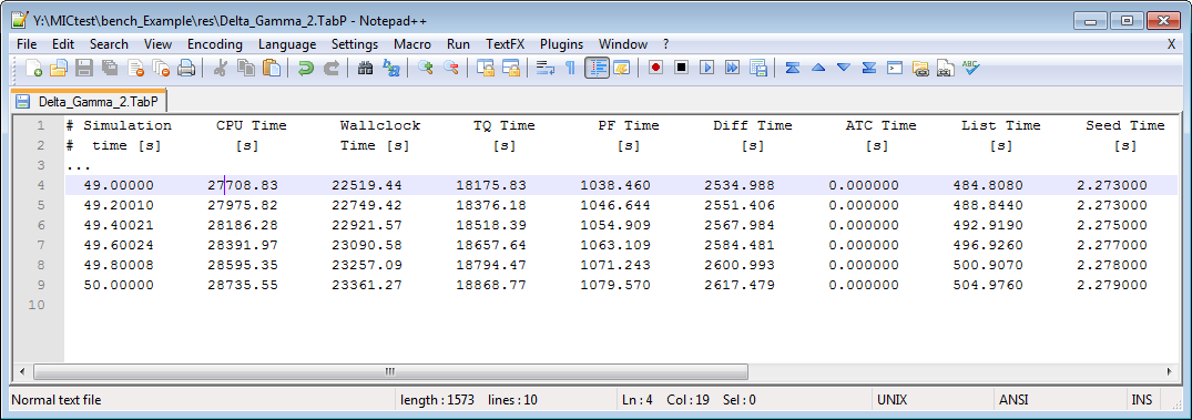
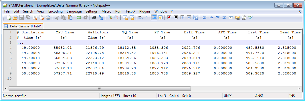
It is possible to reduce the wallclock time of a simulation if the computational load is put heavily on the parallelized solvers. Check the TabP output for getting an impression in which cases you can benefit from using the parallel variants of MICRESS®, see Figure 3. Each line of the text output shows the accumulated time values for the current simulation time step. Except the Simulation Time and CPU Time, all values show wallclock time. The third column, headed with Wallclock Time, shows the overall execution time and reflects the real time gone for the simulation.
Figure 3
Performance Output (TabP)
Two threads
Eight threads
Recommended choices of MICRESS® variants:
-
Serial versions: If there is only little load on the parallelized solvers, it is recommended to use MICRESS® standard serial variants. The parallelization itself introduces some overhead which results in a slow down of the parallel simulation.
-
Parallel versions: Simulation with a fair load on the parallel solvers will benefit from parallel execution with thread counts above 1. The performance will depend on the problem size and the available CPUs on your system when you choose high thread counts. Usually, there is an optimal thread count and the performance degrades beyond.
Example 6
Thread count for accelerating the execution of diffusion, stress, and temperature solvers in parallel MICRESS variants
# Numerical parameters
# ====================
#
...
# Parallel Execution
# ------------------
# Number of parallel threads ?
5
...
-
I. Steinbach, F. Pezzolla, B. Nestler, M. Seeßelberg, R. Prieler, G. J. Schmitz, and J. L. L. Rezende. A phase field concept for multiphase systems. Physica D: Nonlinear Phenomena, 94(3):135–147, jul 1996. doi:10.1016/0167-2789(95)00298-7. ↩↩
-
J. Eiken, B. Böttger, and I. Steinbach. Multiphase-field approach for multicomponent alloys with extrapolation scheme for numerical application. Physical Review, 2006. doi:10.1103/physreve.73.066122. ↩↩
-
Janin Eiken. Numerical solution of the phase-field equation with minimized discretization error. IOP Conference Series: Materials Science and Engineering, 33:012105, jul 2012. doi:10.1088/1757-899x/33/1/012105. ↩
-
B. Böttger, J. Eiken, and M. Apel. Multi-ternary extrapolation scheme for efficient coupling of thermodynamic data to a multi-phase-field model. Computational Materials Science, 108:283–292, oct 2015. doi:10.1016/j.commatsci.2015.03.003. ↩↩↩