Boundary Conditions
The boundary conditions of the simulation domain have to be set for the phase-field variables, the concentration, temperature, fluid flow and displacement fields depending on the type of coupling which has been defined at the beginning. The MICRESS® boundary conditions are defined by a text string with length 4 or 6 which represent a sequence of key characters. The characters specify the type of boundary condition, their sequential order addresses the different sides of the simulation domain (west-east-bottom-top for 2D and west-east-south-north-bottom-top for 3D).
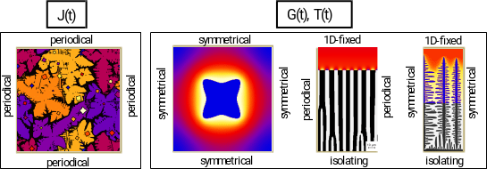
Figure 1
Graphical visualisation of the boundary conditions
The following conditions are available:
-
insulation (
i): The boundary cell (the first cell outside of the simulation domain) is assumed to have the same field value (e.g. phase-field variable) as its direct neighbour (the outermost cell of the domain). The name of the flag reflects the fact that no gradients and, thus, no fluxes exist between the boundary cell and its neighbour inside the simulation domain. -
symmetric (
s): defines the field value of the boundary cell to be identical to its second neighbour in the simulation domain, thus implying a symmetry plane through the centre of the outermost cells of the domain. This condition is similar to an isolation condition which is shifted by half a cell. -
periodic (
p): with this condition, the field value of the boundary cell is set to the value of the outermost cell on the opposite side of the simulation domain. Thus, objects like dendrites which touch one side are continued on the other side. The periodic condition preserves the field balance. -
gradient (
g): the field value of the boundary cell is extrapolated from the first and second neighbour inside the domain. The use of this boundary condition is allowed for all fields (concentration, temperature, phase-field) but not always reasonable. The gradient condition for phase-field is very useful for grain growth. Ifperiodicis not suitable for any reason -- the flaggshould be the best choice for minimising the impact of the boundary condition on the grain structure. Be prepared to get strange effects while usinggwith the concentration field, if phase boundaries are touching the domain boundary! -
fixed (
f): Uses a fixed value for the boundary cell. This value is requested in an extra input line in section Process Condition). Naturally, thefcondition does not preserve the average of the field value. A typical application of the fixed condition for the concentration field is directional solidification with moving frame (fixed condition for top boundary). -
wetting (
w): This option is available only for the phase-field and allows specifying a wetting angle for ... . This value is requested in an extra input line in section Process Condition). .
Example 1
Defining the boundary conditions
...
# Boundary conditions
# ===================
...
# Boundary conditions for phase field in each direction
# Options: i (insulation) s (symmetric) p (periodic/wrap-around)
#          g (gradient)   f (fixed)     w (wetting)
# Sequence: W E (S N, if 3D) B T borders
ppii
#
# Boundary conditions for concentration field in each direction
# Options: i (insulation) s (symmetric) p (periodic/wrap-around) g (gradient) f (fixed)
# Sequence: W E (S N, if 3D) B T borders
ppii
#
...
1D Temperature Boundary Conditions
If the option 1d_temp has been selected at the beginning of the input file (Model - Thermal Conditions), at this place the boundary conditions for the 1D temperature field have to be specified. The user can select between insulation (i), symmetric (s), periodic (p), global gradient (g), fixed (f) and flux (j). While i, s and p have already been explained above, the other conditions are either new or have further implications or a slightly different meaning:
-
global gradient (
g): This condition establishes a given global temperature gradient between the actual boundary and the opposite boundary. This modified gradient condition is especially useful for coupling to external process simulation results: If temperature vs. time and the thermal gradient are known from a macroscopic process simulation (or a corresponding experiment), a time-dependent fixedfcondition (see below) can be applied on one side of the 1D temperature field, and thegcondition on the other side to maintain the gradient. The definition ofgon both sides is not allowed! -
fixed (
f): The definition of this condition corresponds to that of the fixed condition for the normal simulation domain. However, not only a fixed temperature value, but also a temperature-time profile can be read from a text file using thefrom_fileoption. If a constant temperature is chosen, a heat transfer coefficient is additionally requested in section Process Condition), allowing the definition of a heat transfer condition to an external medium with fixed temperature. If the value of the coefficient is \<>=0, the temperature value is used as fixed condition instead. -
flux (
j): This condition allows the assumption of a constant or time-dependent flux [W/cm^2] as boundary condition.
See section Process Conditions for further information about the input of the required thermo-physical data.
Example 2
Defining 1D temperature boundary conditions
...
# Boundary conditions for 1D temperature field bottom and top
# Options: i (insulation) s (symmetric) p (periodic/wrap-around) g (global grad) f (fixed) j (flux)
# Sequence: B T
fi
...
# Process Conditions
# ==================
...
#
# Thermo-physical properties for 1D temperature solver
# ----------------------------------------------------
# How shall temperature in Bottom-direction be read?
# Options:   constant    from_file
constant
# Fixed value for temperature [K]
298.00
# Fixed value for heat transfer coefficient [W/cm2K]
1.5000
#
...
Elastic Stress Boundary Conditions
In case of stress coupling, additional boundary conditions are required. The available options are constant_volume, i.e. zero displacement of all boundaries, free_expansion, i.e. bottom left corner fixed with free expansion in all directions and normal_expansion (formerly parallel_expansion), i.e. bottom left corner fixed, free expansion along main axes. Furthermore, external stress and strain acting on the simulation domain can be defined. The boundary conditions are fix_isostatic_pressure, fix_isostatic_strain, fix_normal_pressure and fix_normal_strain. For the isostatic cases, either the normal pressure at the domain boundaries or the normal displacement are fixed. The values should be specified in a second line (real numbers, units are [MPa] or [\%], respectively). The normal variants allow the definition of normal displacement or normal stress separately in each direction.
Example 3
Boundary Conditions for Elastic Stress Calculation
...
# Boundary condition for elastic stress calculation
# Options: constant_volume  normal_expansion  free_expansion
#          fix_isostatic_pressure  fix_normal_pressure
#          fix_isostatic_strain    fix_normal_strain
fix_normal_pressure
...
Flow Boundary Conditions
If the flow module is activated the user is asked to provide two sets of boundary conditions, one for flow velocity and one for pressure. The available options are listed in the tables below. The 3rd column of the table for pressure boundary conditions lists the velocity boundary conditions that should preferably be combined with a specific pressure boundary condition. If periodic boundary conditions are chosen they should be applied to the opposite boundary as well and to velocity as well as pressure. In this case the user is asked to provide a pressure difference for the boundary pair (see also Flow Solver Boundary Conditions).
Example 4
Example: Flow Boundary Conditions
...
# Boundary conditions for flow field in each direction
# Options: p (periodic) e (in-out) o,+ (in-out normal to wall) f (fixed)
# Options: i (insulation parallel to wall) s (symmetric) l,= (parallel to wall)
# Sequence: W E (S N, if 3D) B T borders
sisiff
#
# Boundary conditions for pressure in each direction
# Options: i (insulation) s (symmetric) n (vonNeumann) p (periodic)
#          g (continuous gradient) f (fixed) - (none, for flow: fisl)
# Sequence: W E (S N, if 3D) B T borders
sisi--
...
For the fixed, symmetric, iso and parallel velocity conditions no condition can be chosen for pressure with a - (dash). The gradient boundary conditions use a linear extrapolation of velocity or pressure on the boundary, to provide a fixed pressure gradient use the neumann boundary condition. Please see section Using the flow solver for more details on flow boundary conditions.
Velocity boundary conditions
| Letter | Meaning |
|---|---|
p | periodic, same velocity as opposite boundary |
f | fixed velocity, provide components in \mu m/s |
s | symmetry plane through cell center |
i | iso, symmetry plane at the boundary |
l,= | parallel, frictionless boundary condition |
o,+ | orthogonal flow to the boundary |
e | free in/out flow |
g | gradient extrapolation of the velocity |
Pressure boundary conditions
| Letter | Meaning | Velocity boundary conditions |
|---|---|---|
p | periodic with fixed offset | p |
f | fixed | o, e, g |
s | symmetric | o, e, g, s |
i | isolated | o, e, g, i, l |
n | neumann, fixed gradient | o, e, g, |
g | gradient extrapolation | o, e, g, f |
- | no boundary condition | f, s, i, l |