Frequently Asked Questions (FAQ)
How to define an initial microstructure
An initial microstructure may be defined as:
deterministic
By determining the amount of grains present at the beginning of the simulation process as well as their exact position and shape. If you choose deterministic grain positioning, you need to define the grain positioning by specifying the x and the z coordinates of each grain in a cartesian coordinate system with an origin the bottom left-hand corner. As far as the grain shape is concerned, you can define round grains by specifying a radius or rectangular and elliptic grains -- by specifying a length axis along the x and the z axes. To describe overlapping grains the Voronoi construction may be used. For more details, refer to chapter Voronoi construction.
random
For random grain definition, you need to specify the total number of grains, the number of different types of grains and the number of grains for each grain type. Then, you specify the geometry for each grain type -- round, elliptic or rectangular. Minimum and a maximum values for the x, y and z coordinates are given to define the region in which the grain centers shall be randomly placed. According to the type of geometry you have chosen for your grains, you need to specify a minimum and a maximum radius for the round grains or minimum and maximum side lengths for rectangular and elliptic grains. Additional to this data a seed for the random generator (integer for randomization) is read in to allow reproducibility. Simulations started at the same computer with the same seed should always reproduce the same initial random structure. Random input is especially helpful to create Voronoi structures with high numbers of grains. To obtain a classic Voronoi structure with straight interfaces, minimal and maximal radii should be set identical. Note that in the case, the effective radii of overlapping grains will be determined by half the distance between the grain centers and not by the specified value of the radius itself. The grain specified radii should be selected high enough to avoid unwanted liquid regions. Different minimal and maximal radii can be chosen to obtain a weighted Voronoi construction with curved interfaces. A too high difference between the radii can however lead to unrealistically round grains. (check chapter Voronoi construction).
from file
By specifying the exact path of the text file containing information about the grain number, grain positioning and grain shape. The number of grains at the beginning can be either specified explicitly or read from the input file. Alternatively, the grain properties can be input directly in the command line, they can set to identical, i.e. all grains have the same properties or they can be divided in blocks, i.e. grain 1 to 3 and grain 4 to 6 if the number of grains was set to 6.
restart structure-only
An initial microstructures may be constructed from the restart output of former simulations. Restarted structures can be shifted, rotated and combined. For high flexibility in locating the individual microstructures, the restart structure is positioned inside the grain of the newly defined structure (defined deterministically or from file). Note that the size of the restart structure has to exceed the size of the grain to be filled.
How to read/include a microstructure file
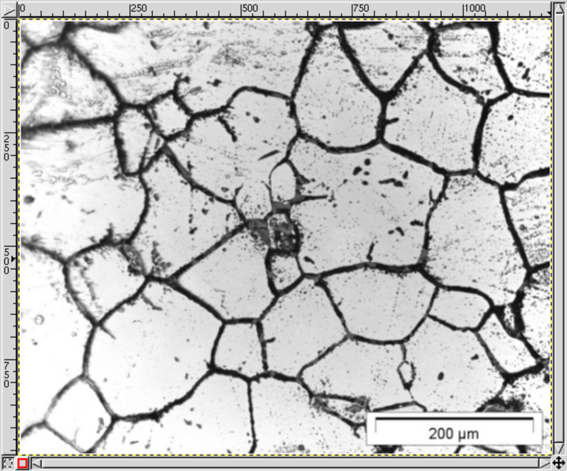
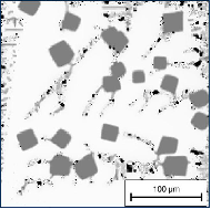
MICRESS® can read initial microstructure and composition or temperature fields from a file. The file to be read should be an ASCII file with a known geometry (number of cells in X and Y direction): the dimension of the read-in data set does not need to be identical to the simulation one. The most complex case is probably reading an experimental grain structure, but this is not as daunting as it could seem.
Here is a step-by-step description how to do that using GIMP (GNU Image Manipulation Program), Version 1.2.5 (www.gimp.org). The micrograph (the first figure from the top) is courtesy of IEHK, RWTH Aachen. Newer GIMP versions have similar functionalities but the naming might differ. However, any full-fledged image manipulation program should support similar procedures.
Remove frames:
- Image → Transform → Zealous Crop
Insert a new foreground layer:
- Layers → New Layer...
Draw the boundaries on the foreground layer:
- Tools → Paint Tools → Pencil
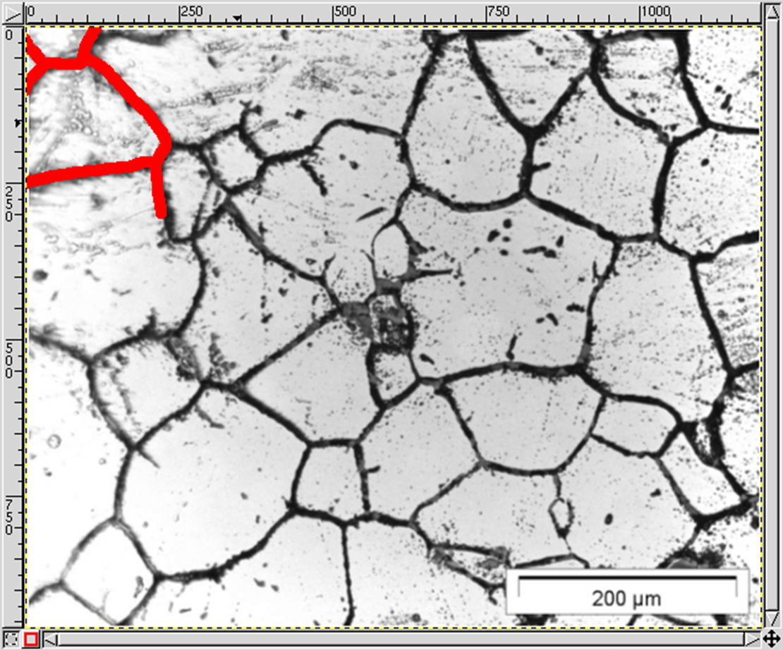
Make sure you do not leave any dangling boundaries, so that each grain is closed (the boundaries of the domain themselves do not have to be re-drawn, as MICRESS will perform this task).
Remove the background layer:
- Layers → Layers, Channels & Paths → Layers
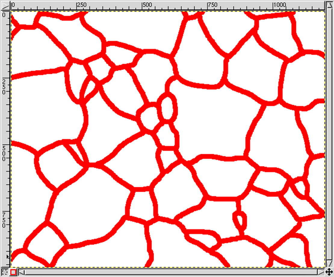
Set the color palette:
- Image → Mode → Indexed
- Enable Black/White (1-Bit) Palette
- Enable No Colour Dithering
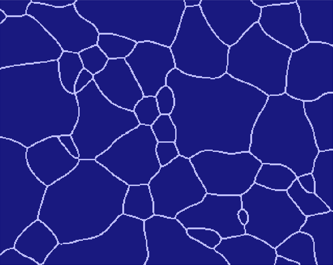
Export file as ASCII PGM (Portable Gray Map):
- File → Export As...
- Append file ending .pgm to filename
- Choose ASCII data formatting
Use the PGM_TO_MICRESS perl script from the 'Tool' directory to proper align the PGM ASCI values according to the picture geometry. The resulting text file can be read by MICRESS.
For some additional information, check section Grain input - From File. You can also check the T020_Grain_Growth_initialFromFile.dri example makes use of reading a microstructure from file.
How to describe an anisotropic/faceted phase
If a phase is defined anisotropic or faceted, all grains of this phase will be assigned with an orientation. You can specify whether the grain orientation shall be defined in terms of 2D-angles, Euler angles, angles/axes pairs or Miller indices. Moreover, you can choose between different crystallographic symmetries. According to the defined crystallographic symmetry, specific orientations will be considered as equivalent. The symmetry is considered when evaluating misorientation-dependent phase interactions and also determines the anisotropy function in case of anisotropic phase interactions. If you define the phase as faceted, you will additionally have to define the facet orientations, i.e. the normal vectors of the facets in the local coordinate system of the grain. Note that facet vectors are not automatically mirrored according to the phase symmetry, but all have to be defined individually. However, facets with equal properties can be grouped to a common facet type. Furthermore, the parameter kappa which determines the broadness of the anisotropy function needs to be specified.
How to include nucleation
To include nucleation and to obtain additional outputs when nuclei are set or a phase disappears, choose the flag out_nucleation in the beginning of the Nucleation section.
Next, the number of types of seeds should be specified. For each seed type a positioning should be given (bulk, in regions, at the interface, at triple or quadruple junctions). If a nucleation region is requested, you should specify its coordinates (in micrometers). After that, specify the phase state of the new grains and the reference phase. The phase of new grain defines the type of seeds (e.g.: Mg2Si intermetallics). The reference phase refers to the kind of phase where the new seeds may appear and from which the undercooling is calculated.
If the interface flag has been selected for the grain positioning, it is necessary to define a substrate phase. This keyword is used for selecting interfaces between this phase and the matrix phase as nucleation sites, as well as and for taking into account the interface curvature in the undercooling calculation. The substrate phase is the one which determines the extra curvature undercooling and the reference phase is then the one where the undercooling is calculated.
Next, the nucleation model to be used for further nucleation is chosen -- the seed density or the seed undercooling model. They have already been presented in input section Nucleation and topic Nucleation Model.
After having chosen the nucleation model to be used in the simulation, MICRESS® asks for a minimum and a maximum nucleation temperature for the different seed types which should lie around the temperature where nucleation is expected.
Noise can be added to the calculation of the driving force for nucleation. In that case, the coefficient for the noise level and a seed for the random number generator will be asked.
One should also specify the maximum number of simultaneous nucleation events to be nucleated in one nucleation check.
In the case of solidification of a pure substance (e.g. T_{melt,Al}=933.55 K) by setting the minimum undercooling to 20 K, one would expect the nuclei to appear at 913.55 K or below. With the help of this flag some stochastic fluctuations are introduced on the undercooling limit.
You can enable the flag kill_metastable to remove metastable grains after their shield time has ellapsed.
The following example with AlSi17Cu4Mg shows how to use the different nucleation modules in a reasonable way:
| Phase | Description |
|---|---|
| primary silicon Si | the seed density model/analytical curvature by default |
| Al dendrite | seed undercooling/stabilisation |
| Si eutectic | interface nucleation/stabilization |
| Mg2Si | interface nucleation/stabilization |
| Al2Cu | interface nucleation/stabilization |
| Al | interface nucleation/stabilization to achieve complete solidification |
How to choose between stabilisation and analytical curvature
Stabilisation
- in the stabilisation model the seed is stabilized by reduction of curvature proportional to phase fraction
- the seed radius must be chosen to be smaller than \Delta x, otherwise a large grain will be set
- the critical seed undercooling must be smaller than critical undercooling corresponding to a radius of \Delta x, otherwise the seed may not grow
- use
kill_metastableto remove such sticking seeds - use this model with seed_undercooling, if initial growth kinetics are less important than stable growth
Analytical curvature
- the curvature is calculated analytically (3D) from the phase fraction of the small grain, with the largest allowed value corresponding to the critical radius
- if a seed radius larger than \Delta x is chosen, the radius corresponds to the largest curvature allowed even after grain increase
- the grain radius is essential for both the curvature and the growth conditions
- mobility is corrected to be as close as possible to real initial kinetics
- use this model for correct description of initial growth or thermal interaction between seeds
- the model is default for the seed-density model
- the model can also be applied for setting initial grains
How to include a further alloy element
In order to include a further alloy element, first you need to change (increase) the number of dissolved constituents in the beginning of the Concentration data section. Further input and corrections of the input file depend on whether you use a TC database coupling or a linearised phase diagram.
- For coupling to a thermodynamic database: add the further alloy element in your database. Make sure that when you run the input file through the command line, there is an additional component appearing. Specify the Thermo-Calc™ index of the new component. Check whether your matrix phase is the right one. Define how diffusion of the new component shall be resolved for the corresponding phases.
- For linearised phase diagrams: define how diffusion of the new component shall be resolved for the corresponding phases. Then, define the dissolved concentration of the new component in the corresponding phases. Moreover, define the two slopes of the new component relative to the already present components at the reference point. Finally, define the initial concentration of the new component in each of the relevant phases present.
For more information you can refer to some of the MICRESS® examples from the MICRESS® installation directory (e.g. T038_Stress.dri, T003_AlCu.dri, T032_P_Peak_2D.dri).
How to add a further phase
Consider the T001_Delta_Gamma.dri example that you have obtained with your installation files. In this example, we will add cementite as a further phase into the simulation. You need to consider the following:
- modifications are necessary at several positions in the .dri file
- cementite should be considered as isotropic and stoichiometric (Fe3C)
- a cementite spherical grain (e.g. d=30 \mu m is placed in the middle of the simulation domain as an initial condition
- the output times should be modified to resolve the dissolution of cementite
- control the traces of cementite in the C-field even after it has dissolved i.e. disappeared from the .phas file
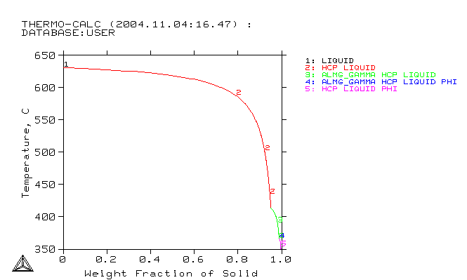
A Thermo-Calc Scheil calculation
How to create .ges files for TC-coupled simulations (overview)
In order to create a GES (Gibbs Energy System) file from thermodynamic database, see the provided Thermo-Calc™ macro example HOWTO_FeCMn.TCM in the Training Examples folder as a reference. This is a normal text file.
Thermo-Calc macro example
...
@@select thermodynamic database
@@ GOTO_MODULE DATABASE_RETRIEVAL
goto dat
@@
@@for example TCFe6 iron and steel database
@@ SWITCH_DATABASE TCFE10
sw TCFe10
@@
@@which list the database elements
@@ LIST_DATABASE elements
l-d elements
@@
@@define elements in alloy systems
@@ DEFINE_SYSTEM fe c mn
d-sys fe c mn
...
Comments are starting with @@. All other lines contain commands for the Thermo-Calc™ console. They can be executed as a complete macro file, e.g. by calling Thermo-Calc with the macro file as parameter, or step-by-step in the console itself.
Thermo-Calc graphical user interface: Console Mode
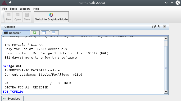
To begin with, select a thermodynamic database (example: TCFe10 iron and steel database). Define the elements in the alloying system and list the system. Next, define the phases of interest. As soon as you are ready with that, get the defined system into the GES-Workspace and repeat the performed steps. Go to the Gibbs workspace and save it to file (example: FeCMn.ges5).
For further details, see the next section How to perform a TC-coupled simulation.
Notes
With version TC 2020a, Thermo-Calc introduced a new GES6 module. Stored GES files still remain version 5 and are compatible to MICRESS.
How to perform a TC-coupled simulation
For simulations with coupling to thermodynamic database, you have to:
Select the relevant components and phases in Thermo-Calc™. This means that you should choose important elements which are supported by the database e.g. AZ31: Mg, Al, Zn. Then, you should choose the important phases. For solidification, use the Thermo-Calc™ Scheil and for solid-solid reactions -- the Thermo-Calc™ Equilibrium.
Create GES5-File from database using Thermo-Calc™. The file should contain the same elements as used in MICRESS: MG, AL, ZN. It should also contain at least all phases which will be used in MICRESS®: Liquid, HCP, ALMG_GAMMA, PHI. You should also include mobility data for some phases if available (append database command in Thermo-Calc™ Classic)
Specify all phase interactions. Switch on the most important interactions (e.g. interactions of secondary phases to LIQUID and primary phase (HCP). Leave out complex interactions of minor importance (e.g. ALMG_GAMMA/PHI), especially if stoichiometric phases are involved. Then, the constant-K model is applied (diffusion between phases, but no movement).
Specify all stoichiometric compositions (see Concentration Solver - Stoichiometry and more). Components without solubility range are assigned automatically as stoichiometric. You should also declare stoichiometric all components with restricted solubility range or steep phase diagram slope. Use the stoichiometric option also in case of pseudo-binary demixing: mk \alpha \Delta S \alpha \cdot mk \beta \Delta S \beta < 0. In that case, apply the stoichiometric condition to the phase with higher value of mk \Delta S. The less favourable extrapolation should be compensated by a higher re-linearisation frequency. In case of solidification, an advanced extrapolation scheme can be applied (applies to all definitions after the keyword stoich_enhanced_on). Note that it is not possible to define a phase interaction if any component has no solubility range or steep slopes in both phases (versions before release 5.5: if the component is declared stoichiometric in both phases)! Diagonal extrapolation (interaction) provides a good alternative to stoichiometric conditions in case of pseudo-binary demixing. The Limits keyword can be used to prevent switching between composition sets by setting composition limits in at%.
Next, specify GES5-File in MICRESS input. Give the path and the name of the .GES5 file for thermodynamic and mobility data. Take care of compatibility (TC version). Increase the workspace size if necessary.
Specify re-linearisation conditions. All newly formed interface cells request automatically new local linearisations (can be sufficient if the front is moving fast). It is recommended to specify a complete re-linearisation period. A maximum effective temperature deviation can be specified per phase interaction. In that case, re-linearisation is performed for the whole interface between two grains.
Run MICRESS to get phase and element numbers in database from screen output.
Driving File
# Components
# ==========
...
# The database contains the following components:
#   AL
#   MG
#   ZN
...
# Phases
# ======
# Selection of Phases
# -------------------
# The database contains 4  phases:
#   ALMG_GAMMA
#   HCP
#   LIQUID
#   PHI
...
Specify relation to components and phases in MICRESS
Driving File
...
# A component can be specified by an element symbol,
# user defined name or database index.
# 'end_of_components' will finish the components input.
# Component 0 (main component) ?
MG
# Thermo-Calc index of (MICRESS) component 1?
AL
# Thermo-Calc index of (MICRESS) component 2?
ZN
...
# A phase can be specified by the name or index used in the database
# or by a user defined name.
# 'end_of_phases' will finish the phase data input.
# Name or database index of phase 0 (matrix phase)
LIQUID
# Name or database index of phase 1
HCP
# Name or database index of phase 2
1
# Name or database index of phase 3
4
...
Specify the molar volumes of the phases (see Phase data - Molar Volumes.
Specify a temperature for initial (quasi-) equilibrium. In most cases, the initial temperature is a good choice.
Check the initial linearization parameters in the .log file. There should be no extreme values (stoichiometric components?). For stoichiometric phases without solubility range, -999.99 will be displayed as a slope. Furthermore, check whether there is any de-mixing mk \alpha \Delta S \alpha \cdot mk \beta \Delta S \beta < 0. Make sure that the initial components are reasonable. If a phase is not present at the beginning, linearization parameters will be calculated when nucleation is checked for the first time.
Hints for troubleshooting:
- most numerical problems in MICRESS® make first Thermo-Calc™ complain! Check mobilities (start always with small values, check .driv output), resolution, etc.
- make sure to declare properly all stoichiometric components! Check the initial linearization output at initialisation or before first nucleation of a new phase (.log file). The initialisation of the phase equilibria can be controlled by the temperature for initial equilibrium or by manual input of initial compositions
- watch out for de-mixing effects (different slopes in solidus and solvus) or slopes near 0. Defining suitable phases/components as stoichiometric can prevent numerical problems at the cost of a more frequent re-linearisation
- check interface per interface by deactivating the other ones (no_phase_interaction)
- use
no_phase_interactionif no driving force can be calculated (e.g. if both phases have no or a very small solubility range for the same component or if linearisation fails). Then, the interface will not move but allow diffusion between the phases - in case of a miscibility gap, separate phase description into composition sets (using Thermo-Calc™), which can have different phase numbers in MICRESS®
- extremely small solubility (e.g. N in fcc at lower temperatures) can cause numerical accuracy problems! Use a double precision MICRESS® version and a small value for phMin.
How to go 3D
You can change the simulation from 2D to 3D by modifying the input file. For that purpose, you need to go to the section: Flags and settings → geometry and then add an integer value > 1 for CellsY. This will define the number of cells in the 3rd dimension.
Further modifications are necessary for the grain orientations i.e. switching from angle 2D to a suitable 3D description.
Also the description of the positions of all grains being set deterministically to define an initial microstructure have to be complemented by the information about the 3rd dimension.
Further, all boundary conditions have to be altered to the respective 3D descriptions.
You should check whether the simulation runs. If you not wish to overwrite the existing input file, you should change the corresponding settings under the Restart options.
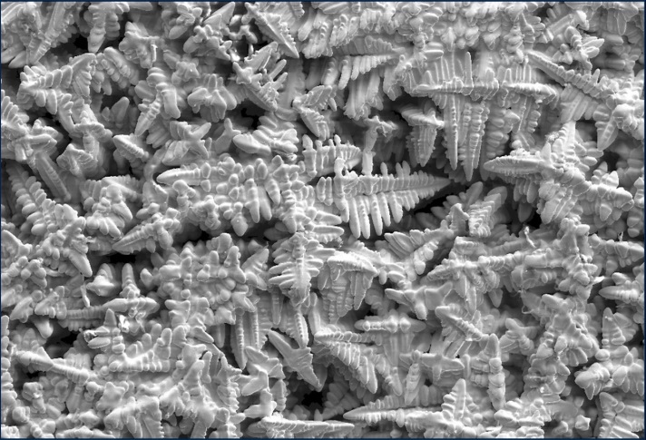
Experimental 3D dendrites prepared by removing the melt by centrifugal force
How to understand and model solidification
Solidification of metallic alloys is an important application for phase-field simulations. The dendritic growth structure is a result of self-organization of the unstable solidification front with a very weak trigger given by the interfacial energy anisotropy. Phase-field simulations capture the underlying physics and make it tractable on a computer. According to the Gibbs--Thomson relation, solidification problems are characterised by:
- the interface velocity coupled to redistribution of heat and solute at the interface
- long-range transport in the bulk phases (Stefan problem)
- interfacial anisotropy is weak and, in good approximation, can be treated as a perturbation of a spherical Wulff shape
- negligible stresses develop on the interface during growth even if solid and liquid differ in density
- heat conduction in both phases is nearly identical
- solute diffusion in solid can be neglected in comparison with solute diffusion in the melt
Issues in dendritic solidification that raise the interest for their modelling at the current stage are:
- the solidification front growing into an undercooled melt is intrinsically unstable and a dendrite can be viewed as a self-organizing structure
- convection in the melt. This is difficult to treat analytically or numerically, but unavoidable under terrestrial conditions
- the analytical solution of steadily growing dendrite approximated by a parabola of revolution is a self-similar solution that does not select the absolute scale, i.e. it fails to predict the scale of the solidification microstructure whereas nature correlates the scale of the microstructure to the material and process conditions well
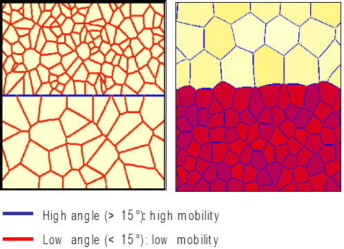
How to perform sub-grain modelling
According to the theory, nucleation of recrystallized grains is almost abnormal growth of sub-grains.
Modelling scenario for sub-grain growth using high- and low-angle grain boundaries
The input given in the following example may be helpful:
Driving File
...
# Geometry
...
# Grain input
# ===========
# Type of grain positioning?
# Options:  deterministic   random   from_file
random
# Integer for randomization?
234567
# Number of different types of grains?
2
# Number of grains of type 1?
14
# Number of grains of type 2?
72
# Input for grain type 1
# -----------------------------
# Geometry of grain type 1
# Options:  round     rectangular    elliptic
round
# Minimal value of x-coordinates?  [micrometers]
0.
# Maximal value of x-coordinates?  [micrometers]
300.
# Minimal value of z-coordinates?  [micrometers]
0.
# Maximal value of z-coordinates?  [micrometers]
150.
...
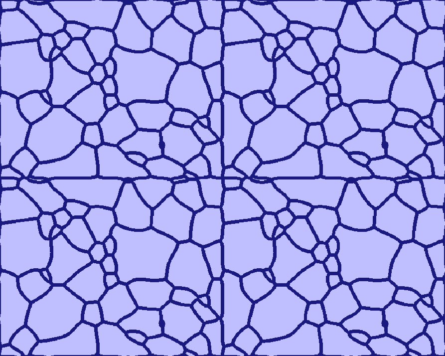
How to handle grains touching the boundaries
Grains touching the boundaries will be closed, so that they do not get merged with others. The user is not restricted in the choice of boundary conditions: even wrap-around, though initially leading to somewhat unexpected grain structures, subsequently allow proper relaxation (see the four-folded symmetry view of the Grain_Growth standard example (T020) below).
A four-folded symmetry view of the "Grain Growth" standard example (T020)
| Early stage | Intermediate stage | Later stage |
|---|---|---|
 | 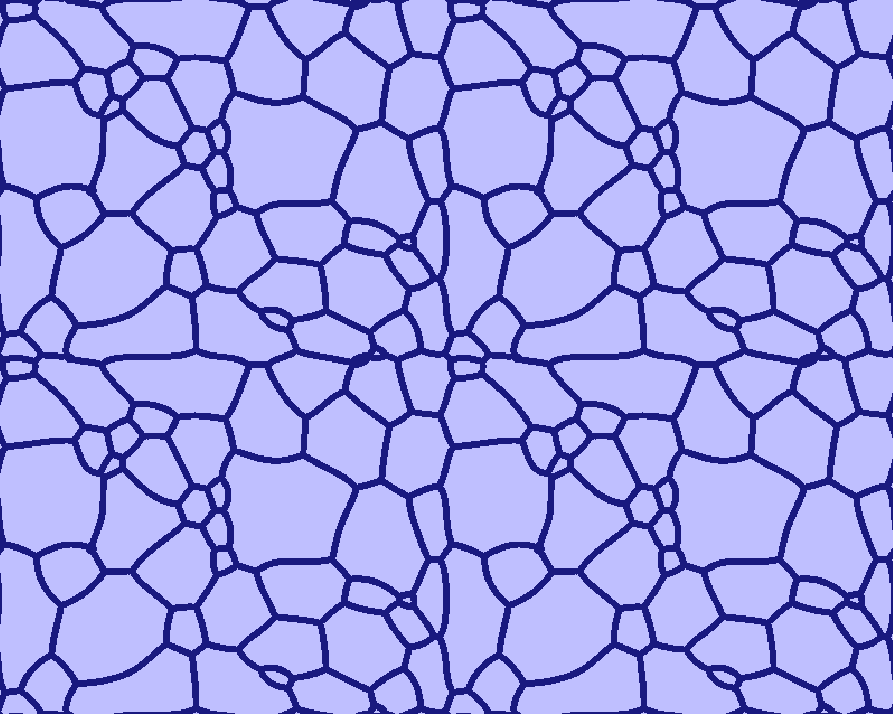 | 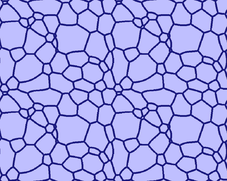 |
How to consider volumetric change
A special model extension allows considering temperature or phase transformation related shrinkage or expansion in concentration coupled simulations. The model conserves matter and is based on the simplifying assumptions that the whole simulation domain expands homogenously while always remaining in a stress-free state. It is activated by specifying concentration volume_change as type of coupling at the beginning of the simulation (see input section Model).
Local volume differences are meant to be instantaneously homogenized by internal material fluxes which are calculated by a newly implemented expansion-relaxation-solver. The local expansion is calculated as product of the local number of moles and the local molar volume, divided by the initial volume. All three quantities can be monitored in respective output files: expansion (*expa), number of moles (*mole) and molar volume (*molV).
During simulation, the local molar volume in each grid cell is evaluated by weighting the phase-specific molar volumes with the local phase fractions. The required phase-specific molar volume data can either be specified by manual input or evaluated from a coupled thermodynamic database. In both cases an additional extrapolation with temperature and/or mean phase composition can be activated by using the kewords temp-extrapolation and conc_extrapolation (input section Molar Volume).
Furthermore, at the start of the input section Concentration Solver, individual components can be defined as interstitial by using this keyword followed by a phase number and component number(s). In contrast to substitutional diffusion, diffusion of interstitial components changes the local number of moles.
Finally, a maximal number of calls per time step and a convergence value have to be specified to control the expansion-relaxation solver. The task of this solver is to homogenize local expansion by compensating material fluxes. The solver runs iteratively and stops when either the specified number of calls per times step is reached or when the mean difference in local expansion falls below the specified convergence value. The effectivity of the solver can be checked by monitoring the degree of homogenization in the expansion output file. The consumed CPU-time is listed in the *TabP file (row: expansion time).
The volume_change model proved to be essentially important for the simulation of spheroidal graphite growth in ductile cast-iron which is driven by interstitial diffusion of carbon through austenite. The attachment of carbon atoms to the graphite interface results in a strong local expansion and a pushing of the surrounding austenitic shell. Simulation of this process without consideration of the volume change would lead to wrong phase volumes, delayed transformation kinetics and artificial segregation effects. Two respective example files are provided: T008_CastIronNodule.dri and T009_CastIronDendriteNodule.dri.