Flow
The following examples demonstrate how to use the flow solver. To simplify matters only phase field coupling is switched on and the phase field is made static by reducing the mobility. The phase field solver is only used at the beginning of the simulation, to generate a phase field profile from the sharp interface. B017_Flow_Cylinder_Karman and T030_Flow_Cylinder_Laminar demonstrate some features of the flow solver at the case of fluid flow around a static cylinder. A009_Flow_Permeability example shows the practical application of calculating the permeability for a given dendritic structure.
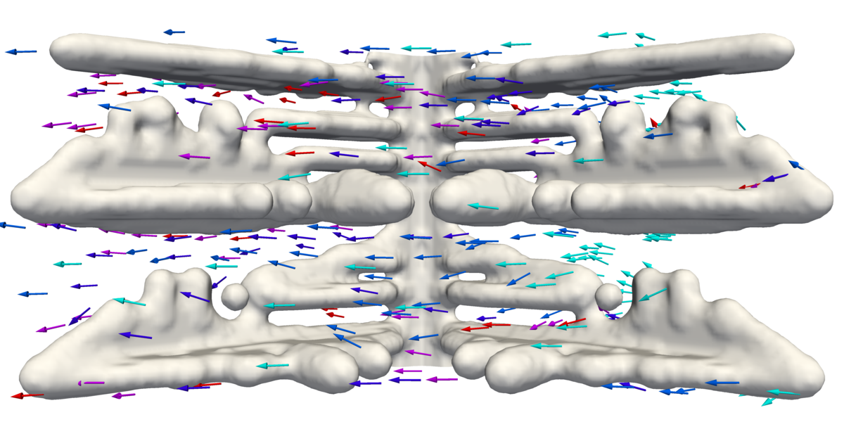
Figure 1 Flow through a dendritic structure
Laminar flow around a cylinder
In this case conditions were chosen so that a stationary, laminar flow around a cylinder results. The fluid flow is driven by the difference between the fixed pressures at in- and outflow. Under these conditions flow is accelerated until frictional forces compensate the driving forces. Frictionless (or gradient) boundary conditions at the top and bottom walls should be avoided here, since they would lead to unphysical situations with unending acceleration. The choice of boundary conditions has an impact on convergence and performance, for larger velocities (resulting from higher pressure gradients) the time steps must be smaller.
Since a stationary, laminar flow with Re \ll 1 is expected the combined solver is used. The time step size was determined in test runs. For the convergence criteria a limit of 10^{-2}/s is set for the continuity equation, matching limits for velocity and pressure are found by observing convergence in tests with higher verbosity. A value of 0.97 for pressure underrelaxation is usually a good choice with the combined solver.
Formation of a Karman vortex street
This is an example of a dynamically changing flow pattern resulting from a stationary geometry. This may happen when the Reynolds number is of O(10) or higher (depending on the geometry). In this case an inlet with a fixed velocity and an outlet with a fixed pressure are set.
For this example the piso solver is employed because of the higher Reynolds number. For time stepping a CFL limit (for C_{adv}) of 0.3 is used. Convergence criteria are chosen to match for a limit of 10^{-1}/s for the continuity equation. In this example the symmetric starting conditions result in a symmetric, nearly static state early in the simulation until breaking of symmetry leads to dynamic changes and finally Karman vortex shedding. Notably convergence behaviour changes when the flow pattern changes, so the convergence criteria must be adjusted to work for the vortex pattern.
Permeability example
This is a demonstration of evaluating the permeability for a 3D structure read in from an ascii VTK file. This file contains, after a header describing the contents, a series of ones and zeroes marking cells as grain 1 (solid) or grain 0 (liquid). Such files can be produced with DP_MICRESS. Another way is to produce legacy VTK output from ParaView (under Data→Save Data). In this case it may be necessary to apply an image resampling filter first (with the x, y and z cell count) to generate data on a structured grid.
Note
Other filters hat may prove helpful:
transformfor symmetry operations,append datasetsto combine mirrored datasets with the original,calculatorto generate the grain number (e.g. from phase fractions) andpass arraysto select only the desired output array.
Since MICRESS® expects cell centred coordinates it may be necessary to edit the header as shown in Figure 2. After the grains are read in as grain structure the profile is adjusted to generate a smooth profile from the sharp interface (but blocky) grain structure. The solid fraction achieved in this way should be checked in the MICRESS® generated output to check if it matches the input structure with sufficient accuracy and possibly adjust the input structure (e.g. by using another threshold when marking cells as solid).
Note
Profile adjustment can take some time for large structures, so you might want to generate a restart file with adjusted profile and start from there (with
steady_restartor frozen phase field) when adjusting convergence parameters.
The steady start option is employed to establish the flow pattern at time step 0. With this option MICRESS® tries to determine a large value for the time steps used to establish a steady pattern (for these steps the time limits do not apply). The number of preliminary time steps is chosen with the pre_iter option, it should be large enough to establish a steady fluid flow pattern. When this is the case the final time steps converge very fast, so verbosity should be kept at 2 for verification.
In some cases the automatic time steps may become too large to achieve convergence, especially when eddies are forming. If this is the case freeze the phase field as in the cylinder examples, start with small time steps and converge the flow pattern in successive runs using restarts while adjusting time steps and convergence parameters.
Figure 2 Changes to present
POINTdata asCELLdata.
# vtk DataFile Version 3.0
vtk output
ASCII
DATASET STRUCTURED_POINTS
DIMENSIONS 199 100 100
SPACING 1 1 1
ORIGIN 0 0 0
POINT_DATA 1990000
SCALARS solid double
LOOKUP_TABLE default
0 0 0 0 0 0 0 0 0
...
# vtk DataFile Version 3.0
vtk output
ASCII
DATASET STRUCTURED_POINTS
DIMENSIONS 200 101 101
SPACING 1 1 1
ORIGIN 0 0 0
CELL_DATA 1990000
SCALARS korn float
LOOKUP_TABLE default
0 0 0 0 0 0 0 0 0
...
Simulation conditions
| Example | A009_Flow _Permeability | B017_Flow _Cylinder_Karman | T030_Flow _Cylinder_Laminar |
|---|---|---|---|
| Dimension | 3-D | 2-D | |
| Grid size | 199x100x100 cells | 200x75 cells | 200x100 cells |
| Grid spacing | 1 microns | 0.5 microns | |
| Interface thickness | 2.5 cells | 5 cells | |
| Boundary conditions |
|
|
|
Results
In Figure 3 the flow patterns caused by a cylindrical object are compared for two different Reynolds numbers. For low Reynolds numbers a very simple stationary pattern occurs, at higher Reynolds numbers eddies will form behind the obstacle, and at even higher Reynolds numbers periodically changing patterns like a Karman vortex street may evolve after some simulation time.
Figure 3 Flow around a cylinder
Re = 1.6 \cdot 10^{-2}
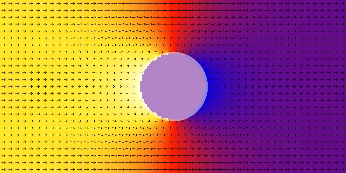
Re = 100
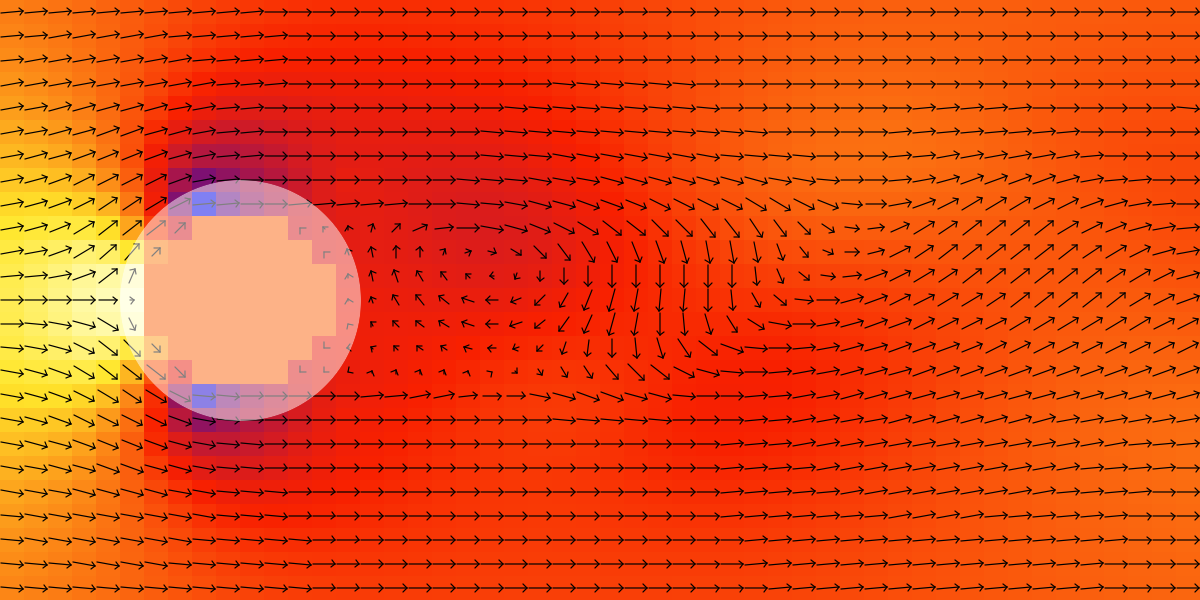
The white circle indicates the grain geometry from the driving file. In the Karman example the grid distance is quite large, so the interaction of melt flow with the phase field interface can be seen: The solid fraction has a braking effect on the fluid flow, so melt flow can pass (tangentially) through the phase field interface but is slowed down.
For the dendritic structure the simulation yields a steady velocity field with an average velocity v_x = 2.8 \cdot 10^{-5} m/s. The average pressure gradient g given in the input equals the pressure difference over the length in x direction.
The dynamic viscosity from the material data section for fluid flow is given by the kinematic viscosity at the density \mu = ν \cdot \rho = 7 \cdot 10^{-3} kg/ms.
From these values the permeability results as k = \frac{\mu \cdot v_x}{g} = 3.9 \cdot 10 ^{-11} m^2.
The value for the liquid fraction of the simulation domain is provided in the tabulated fractions as 84%.