Introduction
MICRESS is a software based on the phase-field method which is considered to be the most appropriate numerical approach for bridging the length scales between the interface capillarity length of a few nanometres and the millimetre scale of diffusion. The phase-field method is a powerful approach to simulate microstructure evolution in the field of material science and engineering.12 The introduction of so-called phase-fields as extra degrees of freedom, additional to temperature and composition allows handling of non-equilibrium processes. This enables simulation of technical processes far from thermodynamic equilibrium, involving kinetic and curvature undercooling, as well as supersaturation.3 A characteristic feature of the phase-field model is the diffusiveness of the interfaces, which are described by a steep but continuous transition of the phase-field variable from one to zero. This avoids a direct tracking of the interface position and essentially facilitates the handling of complex multidimensional morphologies.
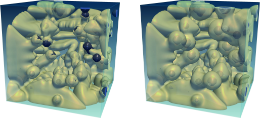
3D phase-field simulations of graphite growth in ductile cast iron
The software addresses technical microstructures which commonly consist of multiple phases, separated by phase boundaries. These phase regions may further be divided into grains, i.e. regions of different crystallographic orientation, separated by grain boundaries. The multiphase-field model implemented in MICRESS most generally defines distinct phase-field parameter for each grain of each phase involved. The phase-field parameters describe the fraction of the associated grain as a continuous function of space and time. The evolution of the phase-fields with time – and implicitly the motion of the phase interfaces and grain boundaries – is described by a set of coupled partial differential equations. These equations are derived from a free energy functional based on a relaxation approach. Note that in contrast to an earlier simplified formulation of the multiphase-field method4, the present multiphase formulation35 has been consistently derived from a common free energy functional and correctly handles local equilibrium and dynamics in higher order interface junctions. The total set of phase-field equations is solved explicitly by the finite difference (FD) method on a regular grid. A dedicated FD correction scheme67 allows for high accuracy for even for small numbers of interface cells. The set of phase-field equations can be solved in combination with diffusion equations for concentration or temperature with a great choice of different various nucleation and boundary conditions. Moreover, stress and flow fields can be considered.
Microstructure evolution is essentially governed by thermodynamic driving forces, diffusion and curvature. The required thermodynamic data of alloys can either be provided to MICRESS in the form of locally linearised phase diagrams or by direct coupling to thermodynamic data sets via a special TQ interface (developed in collaboration with Thermo-Calc AB, Stockholm, Sweden). Furthermore, diffusion data can be derived from coupled chemical mobility databases. While manual input of constant or linearized data is helpful for fundamental academic research, database coupling is highly recommended for all practical applications. Specially developed internal extrapolation schemes enable an efficient treatment of the multicomponent multiphase thermodynamics in between the frequent updates.58
The MICRESS software can be used for a variety of applications and processes covering solidification, solid state transformations, grain growth, recrystallization, heat treatment and much more. The time- and space-resolved simulations can be performed in 1-D, 2-D or 3-D. The size of the simulation domain, the number of grains, phases and components can freely be chosen, but are of course restricted by the available memory size and CPU time. A number of integrated sub-models allow for a flexible choice of nucleation and boundary and thermal conditions.910
Features
MICRESS handles:
- 1-D, 2-D or 3-D calculation domains with free choice of size and resolution
- materials with arbitrary number of components, phases and grains
- solidification, solid-state transition, grain growth, recrystallization, etc.
- complex multicomponent multiphase thermodynamics and diffusion
- anisotropy of phase interfaces and grain boundaries
MICRESS allows for:
- individual definition of bulk properties for each phase
- individual definition of interface properties for phase interactions
- input of properties and process conditions obtained from experiment
- flexible choice of nucleation and boundary conditions
- great choice of output evaluation
MICRESS supports:
- coupling to thermodynamic databases (via the Thermo-Calc™ interface)
- coupling to chemical mobility databases
- coupling to stress and strain module
- coupling to flow module
- Integrated Computational Materials Engineering (ICME)
Model
The phase-field equation implemented in MICRESS software reads
Equation 1
where, \alpha, \beta, \gamma, and \upsilon represent three different grains, and the number of grains in the system, respectively; the subscripts \alpha \beta and \alpha \beta\gamma represent the interface between grains \alpha and \beta and the triple point junction between grains \alpha\beta\gamma, respectively.
On the right-hand side of the above equation, M_{\alpha \beta}^{\phi} and the terms inside the brackets represent the phase-field mobility of the interface \alpha \beta and the net force acting on that interface, respectively. Inside the brackets, the first, second, and third terms represent the thermodynamic, capillarity, and high order junction forces, respectively. In the second term, {\sigma_{\alpha \beta}}, K_{\alpha \beta}, and A_{\alpha \beta} represent the anisotropic interfacial energy, pairwise curvature, and anisotropy of the interface \alpha \beta, respectively; finally, the last term represents the higher order junction forces at the triple point junction \alpha, \beta, and \gamma.
In this section, relations that are required to calculate the different quantities on the right hand side of the phase-field equation are discussed .
The phase-field mobility M_{\alpha \beta}^{\phi} is related to the kinetic coefficient in the Gibbs-Thomson equation (also known as the sharp interface mobility) \mu_{\alpha \beta}^{G} through 11
Equation 2
where \eta is the thickness of the interface in phase-field simulations, {\Delta}s_{\alpha \beta} is the entropy of fusion between the phases of grains {\alpha} and {\beta}, m_{i}^{l} is the slope of the liquidus line for component i, D_{\alpha}^{\text{ij}} is the diffusion matrix for grain {\alpha}, k_j is the partition coefficient. For a pure material, or in the limit of {\eta} ---> 0, the second term in the denominator will be zero and the equation will reduce to {M}_{\alpha \beta}^{\phi} =\ \mu_{\alpha \beta}^{G}. For alloys and when {\eta} is finite, the equation will result in a phase-field mobility that is smaller than the sharp interface mobility.
In Equation 1, b in the first term inside the brackets on the right-hand side is a pre-factor, which is calculated from
Equation 3
In Equation 1, {\Delta G}_{\alpha \beta} is calculated from a relation that is derived in the appendix and reads
Equation 4
The pairwise curvature term K_{\alpha \beta} is calculated from
Equation 5
The high order triple junction term J_{\alpha \beta\gamma} is calculated from
Equation 6
Appendix
Before discussing how the term {\Delta G}_{\alpha \beta} is defined and calculated, the definitions of the mixture quantities and chemical and diffusion potentials need to be introduced.
These potentials are both denoted by the symbol \mu. To distinguish between them, the diffusion potential will have a "~". These potentials can be defined for a phase and also for the mixture of phases. In the former case, the symbol will take a subscript that denotes the phase, while in the latter case, there will be no subscripts. Potentials of different components will be distinguished from each other by a superscript that denotes the component. Next, the mathematical definitions of these potentials are introduced.
The chemical potential of component i in phase \alpha, \mu_{\alpha}^{i}, is defined as the increment in the Gibbs free energy of the phase \alpha, G_{\alpha}, when a very small moles of species i, n^{i}, is added to that phase, while all other variables of the phase are kept constant. The definition is mathematically expressed as
Equation 7
The diffusion potential of the species i in the mixture, {\widetilde{\mu}}^{i}, is defined as the increment in the molar Gibbs free energy density of the mixture g, when the concentration of the species i, c^{i}, is incremented, while all other variables of the mixture are kept constant. The definition is mathematically expressed as
Equation 8
Similarly, the diffusion potential of the species i in phase \alpha, {\widetilde{\mu}}_{\alpha}^{i}, is defined as the increment in the molar Gibbs free energy density of the phase, g_{\alpha}, when the concentration of the species i in the phase \alpha, c_{\alpha}^{i}, is incremented, while all other variables of the phase are kept constant. The definition can be mathematically expressed as
Equation 9
Next, it is shown that, for any component in the system, the difference between the chemical and diffusion potentials of any phase is equal to the chemical potential of the solvant in that phase. The gibbs free energy and concentration of the mixture are defined as
Mixture Quantities
Equation 10
Equation 11
Equation 12
where k and \nu represent the number of components and phases in the system, respectively; the first and second equalities follow from the definition of molar Gibbs free energy and \mu_{\alpha}^{i} (i.e., Equation 7), respectively.
Note that the concentration of component i in phase \alpha, c_{\alpha}^{i}, is defined as the mole number of the component in the phase divided by the total number of moles in that phase (i.e., c_{\alpha}^{i} \equiv \frac{n_{\alpha}^{i}}{n_{\alpha}}), n_{\alpha}^{i}; therefore, in Equation 12, n_{\alpha}^{i} can be replaced with n_{\alpha}c_{\alpha}^{i}, and the equation can be re-written as
Equation 13
The sum of concentration of different components in phase \alpha is, obviously, equal to unity: \sum_{i = 0}^{k}c_{\alpha}^{i} = c_{\alpha}^{0} + \sum_{i = 1}^{k}c_{\alpha}^{i} = 1. Using that equality to eliminate c_{\alpha}^{0} (on the right hand side of the third equality) in Equation 13 gives
Equation 14
Now, from the first equality in Equation 12 and the second equality in Equation 14, one can write
Equation 15
Taking the derivate of both sides of Equation 15 with respect to c_{\alpha}^{i} gives
Equation 16
Substituting the left-hand side of Equation 16 from the definition of the diffusion potential within phase \alpha (i.e., Equation 9) and re-arranding the result gives
Equation 17
whihc, as already stated at the begining of this section, states that, for any component, the difference between the chemical and diffusion potentials at any phase are the same and equal to the chemical potential of the solvant in that phase.
Now that the definition of different potentials are introduced and the relation between chemical and diffusion potentials are derived, the definition of the thermodynamic driving force and its calculation is discussed. The force is defined as
Equation 18
where f is the volumetric free energy, which is related to the molar free energy g as
Equation 19
Substituting Equation 19 into Equation 18 gives
Equation 20
To calculate the derivatives on the right-hand side of this equation, first the Gibbs free energy needs to be expanded as
Equation 21
where \overrightarrow{\widetilde{\mu}} is a vector that contains the diffusion potentials of the different system components in the mixture, \overrightarrow{\widetilde{\mu}} = \left\{\widetilde{\mu}^{i}\right\}_{i: 1...n_{c}} and, as already discussed in connection with Equation 8, \widetilde{\mu}^{i} is the diffusion potential of component i in the mixture.
Taking the derivative of Equation 21 with respect to the phase-fractions \phi_{\alpha} and \phi_{\beta} gives
Equation 22
Equation 23
Substituting Equation 22 and Equation 23 into Equation 20 gives
Equation 24
The three terms inside the brackets are expanded as
Equation 25
Equation 26
Equation 27
Substituting equations 25 to 27 into equation 24 gives
Equation 28
where the second equality follows simply from canceling out the identical terms of the left-hand side of that equality, and the third equality follows from equations 17.
Quasi-Equilibrium
If one assumes that the mass transport between the different phases that co-exist at the interfacial region is fast enough such that the changes in the local c_{\alpha} are much higher than the changes in the local \phi_{\alpha} and c, then those latter changes can be disregarded. Therefore, the local free energy can be minimized by the changes in c_{\alpha} only, and the minimum in free energy is reached when \frac{\partial g}{\partial c_{\alpha}^{i}} = 0.
To express the concept mathematically, one needs to take the derivative of equation 21 with respect to c_{\alpha}^{i} to get
Equation 29
where the second equality follows from equation 9, and then set the result to zero to get
Equation 30
Note that this equation indicates that the diffusion potential of any component in different phases are equal:
Equation 31
Finally, substituting equation 31 into equation 28 gives
Equation 32
References
-
Ingo Steinbach. Phase-field models in materials science. Modelling and Simulation in Materials Science and Engineering, 17(7):073001, jul 2009. doi:10.1088/0965-0393/17/7/073001. ↩
-
Nele Moelans, Bart Blanpain, and Patrick Wollants. An introduction to phase-field modeling of microstructure evolution. Calphad, 32(2):268–294, jun 2008. doi:10.1016/j.calphad.2007.11.003. ↩
-
Janin Eiken. A Phase-Field Model for Technical Alloy Solidification. RWTH Aachen University, 2009. ISBN 9783832290108. ↩↩
-
I. Steinbach, F. Pezzolla, B. Nestler, M. Seeßelberg, R. Prieler, G. J. Schmitz, and J. L. L. Rezende. A phase field concept for multiphase systems. Physica D: Nonlinear Phenomena, 94(3):135–147, jul 1996. doi:10.1016/0167-2789(95)00298-7. ↩
-
J. Eiken, B. Böttger, and I. Steinbach. Multiphase-field approach for multicomponent alloys with extrapolation scheme for numerical application. Physical Review, 2006. doi:10.1103/physreve.73.066122. ↩↩
-
Janin Eiken. Numerical solution of the phase-field equation with minimized discretization error. IOP Conference Series: Materials Science and Engineering, 33:012105, jul 2012. doi:10.1088/1757-899x/33/1/012105. ↩
-
Janin Eiken. The finite phase-field method - a numerical diffuse interface approach for microstructure simulation with minimized discretization error. MRS Proceedings, 2011. doi:10.1557/opl.2012.510. ↩
-
B. Böttger, J. Eiken, and M. Apel. Multi-ternary extrapolation scheme for efficient coupling of thermodynamic data to a multi-phase-field model. Computational Materials Science, 108:283–292, oct 2015. doi:10.1016/j.commatsci.2015.03.003. ↩
-
B. Böttger, J. Eiken, and I. Steinbach. Phase field simulation of equiaxed solidification in technical alloys. Acta Materialia, 54(10):2697–2704, jun 2006. doi:10.1016/j.actamat.2006.02.008. ↩
-
B. Böttger, J. Eiken, and M. Apel. Phase-field simulation of microstructure formation in technical castings - a self-consistent homoenthalpic approach to the micro-macro problem. Journal of Computational Physics, 228(18):6784–6795, oct 2009. doi:10.1016/j.jcp.2009.06.028. ↩
-
A. Carré, and B. Böttger, and M. Apel. Implementation of an antitrapping current for a multicomponent multiphase-field approach. Journal of Crystal Growth, 380:5–13, 2013. doi:10.1016/j.jcrysgro.2013.05.032. ↩